%matplotlib inline
import numpy as np
import matplotlib.pyplot as plt
import os, jdc, shutil
from tqdm import tqdm

from rl_glue import RLGlue
from agent import BaseAgent
from maze_env import ShortcutMazeEnvironment

os.makedirs('results', exist_ok=True)
plt.rcParams.update({'font.size': 15})
plt.rcParams.update({'figure.figsize': [8,5]})
Section 1: Dyna-Q
Let’s start with a quick recap of the tabular Dyna-Q algorithm.

Dyna-Q involves four basic steps:
- Action selection: given an observation, select an action to be performed (here, using the $\epsilon$-greedy method).
- Direct RL: using the observed next state and reward, update the action values (here, using one-step tabular Q-learning).
- Model learning: using the observed next state and reward, update the model (here, updating a table as the environment is assumed to be deterministic).
- Planning: update the action values by generating $n$ simulated experiences using certain starting states and actions (here, using the random-sample one-step tabular Q-planning method). This is also known as the ‘Indirect RL’ step. The process of choosing the state and action to simulate an experience with is known as ‘search control’.
Steps 1 and 2 are parts of the tabular Q-learning algorithm and are denoted by line numbers (a)–(d) in the pseudocode above. Step 3 is performed in line (e), and Step 4 in the block of lines (f).
We highly recommend revising the Dyna videos in the course and the material in the RL textbook (in particular, Section 8.2).
Alright, let’s begin coding.
As you already know by now, you will develop an agent which interacts with the given environment via RL-Glue. More specifically, you will implement the usual methods agent_start, agent_step, and agent_end in your DynaQAgent class, along with a couple of helper methods specific to Dyna-Q, namely update_model and planning_step. We will provide detailed comments in each method describing what your code should do.
Let’s break this down in pieces and do it one-by-one.
First of all, check out the agent_init method below. As in earlier assignments, some of the attributes are initialized with the data passed inside agent_info. In particular, pay attention to the attributes which are new to DynaQAgent, since you shall be using them later.
# Do not modify this cell!

class DynaQAgent(BaseAgent):

    def agent_init(self, agent_info):
        """Setup for the agent called when the experiment first starts.

        Args:
            agent_init_info (dict), the parameters used to initialize the agent. The dictionary contains:
            {
                num_states (int): The number of states,
                num_actions (int): The number of actions,
                epsilon (float): The parameter for epsilon-greedy exploration,
                step_size (float): The step-size,
                discount (float): The discount factor,
                planning_steps (int): The number of planning steps per environmental interaction

                random_seed (int): the seed for the RNG used in epsilon-greedy
                planning_random_seed (int): the seed for the RNG used in the planner
            }
        """

        # First, we get the relevant information from agent_info
        # NOTE: we use np.random.RandomState(seed) to set the two different RNGs
        # for the planner and the rest of the code
        try:
            self.num_states = agent_info["num_states"]
            self.num_actions = agent_info["num_actions"]
        except:
            print("You need to pass both 'num_states' and 'num_actions' \
                   in agent_info to initialize the action-value table")
        self.gamma = agent_info.get("discount", 0.95)
        self.step_size = agent_info.get("step_size", 0.1)
        self.epsilon = agent_info.get("epsilon", 0.1)
        self.planning_steps = agent_info.get("planning_steps", 10)

        self.rand_generator = np.random.RandomState(agent_info.get('random_seed', 42))
        self.planning_rand_generator = np.random.RandomState(agent_info.get('planning_random_seed', 42))

        # Next, we initialize the attributes required by the agent, e.g., q_values, model, etc.
        # A simple way to implement the model is to have a dictionary of dictionaries,
        #        mapping each state to a dictionary which maps actions to (reward, next state) tuples.
        self.q_values = np.zeros((self.num_states, self.num_actions))
        self.actions = list(range(self.num_actions))
        self.past_action = -1
        self.past_state = -1
        self.model = {} # model is a dictionary of dictionaries, which maps states to actions to
                        # (reward, next_state) tuples
Now let’s create the update_model method, which performs the ‘Model Update’ step in the pseudocode. It takes a (s, a, s', r) tuple and stores the next state and reward corresponding to a state-action pair.
Remember, because the environment is deterministic, an easy way to implement the model is to have a dictionary of encountered states, each mapping to a dictionary of actions taken in those states, which in turn maps to a tuple of next state and reward. In this way, the model can be easily accessed by model[s][a], which would return the (s', r) tuple.
%%add_to DynaQAgent

# [GRADED]

def update_model(self, past_state, past_action, state, reward):
    """updates the model

    Args:
        past_state       (int): s
        past_action      (int): a
        state            (int): s'
        reward           (int): r
    Returns:
        Nothing
    """
    # Update the model with the (s,a,s',r) tuple (1~4 lines)

    ### START CODE HERE ###
    self.model[past_state] = self.model.get(past_state, {})
    self.model[past_state][past_action] = state, reward
    ### END CODE HERE ###
Test update_model()
# Do not modify this cell!

## Test code for update_model() ##

actions = []
agent_info = {"num_actions": 4,
              "num_states": 3,
              "epsilon": 0.1,
              "step_size": 0.1,
              "discount": 1.0,
              "random_seed": 0,
              "planning_random_seed": 0}
test_agent = DynaQAgent()
test_agent.agent_init(agent_info)
test_agent.update_model(0,2,0,1)
test_agent.update_model(2,0,1,1)
test_agent.update_model(0,3,1,2)
print("Model: \n", test_agent.model)
Model:
 {0: {2: (0, 1), 3: (1, 2)}, 2: {0: (1, 1)}}
Expected output:
Model:
 {0: {2: (0, 1), 3: (1, 2)}, 2: {0: (1, 1)}}
Next, you will implement the planning step, the crux of the Dyna-Q algorithm. You shall be calling this planning_step method at every timestep of every trajectory.
%%add_to DynaQAgent

# [GRADED]

def planning_step(self):
    """performs planning, i.e. indirect RL.

    Args:
        None
    Returns:
        Nothing
    """

    # The indirect RL step:
    # - Choose a state and action from the set of experiences that are stored in the model. (~2 lines)
    # - Query the model with this state-action pair for the predicted next state and reward.(~1 line)
    # - Update the action values with this simulated experience.                            (2~4 lines)
    # - Repeat for the required number of planning steps.
    #
    # Note that the update equation is different for terminal and non-terminal transitions.
    # To differentiate between a terminal and a non-terminal next state, assume that the model stores
    # the terminal state as a dummy state like -1
    #
    # Important: remember you have a random number generator 'planning_rand_generator' as
    #     a part of the class which you need to use as self.planning_rand_generator.choice()
    #     For the sake of reproducibility and grading, *do not* use anything else like
    #     np.random.choice() for performing search control.

    ### START CODE HERE ###
    for i in range(self.planning_steps):
        past_state = self.planning_rand_generator.choice(list(self.model.keys()))
        past_action = self.planning_rand_generator.choice(list(self.model[past_state].keys()))
        next_state, reward = self.model[past_state][past_action]

        if next_state == -1:
            q_max = 0
        else:
            q_max = np.max(self.q_values[next_state])

        self.q_values[past_state, past_action] += self.step_size * (reward + self.gamma * q_max
                                                                    - self.q_values[past_state, past_action])
    ### END CODE HERE ###
Test planning_step()
# Do not modify this cell!

## Test code for planning_step() ##

actions = []
agent_info = {"num_actions": 4,
              "num_states": 3,
              "epsilon": 0.1,
              "step_size": 0.1,
              "discount": 1.0,
              "planning_steps": 4,
              "random_seed": 0,
              "planning_random_seed": 5}
test_agent = DynaQAgent()
test_agent.agent_init(agent_info)
test_agent.update_model(0,2,1,1)
test_agent.update_model(2,0,1,1)
test_agent.update_model(0,3,0,1)
test_agent.update_model(0,1,-1,1)
test_agent.planning_step()
print("Model: \n", test_agent.model)
print("Action-value estimates: \n", test_agent.q_values)
Model:
 {0: {2: (1, 1), 3: (0, 1), 1: (-1, 1)}, 2: {0: (1, 1)}}
Action-value estimates:
 [[0.  0.1 0.  0.2]
 [0.  0.  0.  0. ]
 [0.1 0.  0.  0. ]]
Expected output:
Model:
 {0: {2: (1, 1), 3: (0, 1), 1: (-1, 1)}, 2: {0: (1, 1)}}
Action-value estimates:
 [[0.   0.1   0.   0.2 ]
 [0.   0.   0.   0.  ]
 [0.1 0.   0.   0.  ]]
If your output does not match the above, one of the first things to check is to make sure that you haven’t changed the planning_random_seed in the test cell. Additionally, make sure you have handled terminal updates correctly.
Now before you move on to implement the rest of the agent methods, here are the helper functions that you’ve used in the previous assessments for choosing an action using an $\epsilon$-greedy policy.
%%add_to DynaQAgent

# Do not modify this cell!

def argmax(self, q_values):
    """argmax with random tie-breaking
    Args:
        q_values (Numpy array): the array of action values
    Returns:
        action (int): an action with the highest value
    """
    top = float("-inf")
    ties = []

    for i in range(len(q_values)):
        if q_values[i] > top:
            top = q_values[i]
            ties = []

        if q_values[i] == top:
            ties.append(i)

    return self.rand_generator.choice(ties)

def choose_action_egreedy(self, state):
    """returns an action using an epsilon-greedy policy w.r.t. the current action-value function.

    Important: assume you have a random number generator 'rand_generator' as a part of the class
                which you can use as self.rand_generator.choice() or self.rand_generator.rand()

    Args:
        state (List): coordinates of the agent (two elements)
    Returns:
        The action taken w.r.t. the aforementioned epsilon-greedy policy
    """

    if self.rand_generator.rand() < self.epsilon:
        action = self.rand_generator.choice(self.actions)
    else:
        values = self.q_values[state]
        action = self.argmax(values)

    return action
Next, you will implement the rest of the agent-related methods, namely agent_start, agent_step, and agent_end.
%%add_to DynaQAgent

# [GRADED]

def agent_start(self, state):
    """The first method called when the experiment starts,
    called after the environment starts.
    Args:
        state (Numpy array): the state from the
            environment's env_start function.
    Returns:
        (int) the first action the agent takes.
    """

    # given the state, select the action using self.choose_action_egreedy()),
    # and save current state and action (~2 lines)
    ### self.past_state = ?
    ### self.past_action = ?

    ### START CODE HERE ###
    action = self.choose_action_egreedy(state)

    self.past_state = state
    self.past_action = action
    ### END CODE HERE ###

    return self.past_action

def agent_step(self, reward, state):
    """A step taken by the agent.

    Args:
        reward (float): the reward received for taking the last action taken
        state (Numpy array): the state from the
            environment's step based on where the agent ended up after the
            last step
    Returns:
        (int) The action the agent takes given this state.
    """

    # - Direct-RL step (~1-3 lines)
    # - Model Update step (~1 line)
    # - `planning_step` (~1 line)
    # - Action Selection step (~1 line)
    # Save the current state and action before returning the action to be performed. (~2 lines)

    ### START CODE HERE ###
    # Direct-RL step
    q_max = np.max(self.q_values[state])
    self.q_values[self.past_state, self.past_action] += self.step_size * (reward + self.gamma * q_max
                                                                - self.q_values[self.past_state, self.past_action])
    # Model Update step
    self.update_model(self.past_state, self.past_action, state, reward)
    # Planning
    self.planning_step()
    # Choose Action
    action = self.choose_action_egreedy(state)
    # Save the current state and action
    self.past_state = state
    self.past_action = action
    ### END CODE HERE ###

    return self.past_action

def agent_end(self, reward):
    """Called when the agent terminates.

    Args:
        reward (float): the reward the agent received for entering the
            terminal state.
    """

    # - Direct RL update with this final transition (1~2 lines)
    # - Model Update step with this final transition (~1 line)
    # - One final `planning_step` (~1 line)
    #
    # Note: the final transition needs to be handled carefully. Since there is no next state,
    #       you will have to pass a dummy state (like -1), which you will be using in the planning_step() to
    #       differentiate between updates with usual terminal and non-terminal transitions.

    ### START CODE HERE ###
    # Direct-RL step
    self.q_values[self.past_state, self.past_action] += self.step_size * (reward
                                                                          - self.q_values[self.past_state, self.past_action])
    # Model Update step
    self.update_model(self.past_state, self.past_action, -1, reward)
    # Planning
    self.planning_step()
    ### END CODE HERE ###
Test agent_start()
# Do not modify this cell!

## Test code for agent_start() ##

agent_info = {"num_actions": 4,
              "num_states": 3,
              "epsilon": 0.1,
              "step_size": 0.1,
              "discount": 1.0,
              "random_seed": 0,
              "planning_random_seed": 0}
test_agent = DynaQAgent()
test_agent.agent_init(agent_info)
action = test_agent.agent_start(0)
print("Action:", action)
print("Model: \n", test_agent.model)
print("Action-value estimates: \n", test_agent.q_values)
Action: 1
Model:
 {}
Action-value estimates:
 [[0. 0. 0. 0.]
 [0. 0. 0. 0.]
 [0. 0. 0. 0.]]
Expected output:
Action: 1
Model:
 {}
Action-value estimates:
 [[0. 0. 0. 0.]
 [0. 0. 0. 0.]
 [0. 0. 0. 0.]]
Test agent_step()
# Do not modify this cell!

## Test code for agent_step() ##

actions = []
agent_info = {"num_actions": 4,
              "num_states": 3,
              "epsilon": 0.1,
              "step_size": 0.1,
              "discount": 1.0,
              "planning_steps": 2,
              "random_seed": 0,
              "planning_random_seed": 0}
test_agent = DynaQAgent()
test_agent.agent_init(agent_info)
actions.append(test_agent.agent_start(0))
actions.append(test_agent.agent_step(1,2))
actions.append(test_agent.agent_step(0,1))
print("Actions:", actions)
print("Model: \n", test_agent.model)
print("Action-value estimates: \n", test_agent.q_values)
Actions: [1, 3, 1]
Model:
 {0: {1: (2, 1)}, 2: {3: (1, 0)}}
Action-value estimates:
 [[0.     0.3439 0.     0.    ]
 [0.     0.     0.     0.    ]
 [0.     0.     0.     0.    ]]
Expected output:
Actions: [1, 3, 1]
Model:
 {0: {1: (2, 1)}, 2: {3: (1, 0)}}
Action-value estimates:
 [[0.     0.3439 0.     0.    ]
 [0.     0.     0.     0.    ]
 [0.     0.     0.     0.    ]]
Test agent_end()
# Do not modify this cell!

## Test code for agent_end() ##

actions = []
agent_info = {"num_actions": 4,
              "num_states": 3,
              "epsilon": 0.1,
              "step_size": 0.1,
              "discount": 1.0,
              "planning_steps": 2,
              "random_seed": 0,
              "planning_random_seed": 0}
test_agent = DynaQAgent()
test_agent.agent_init(agent_info)
actions.append(test_agent.agent_start(0))
actions.append(test_agent.agent_step(1,2))
actions.append(test_agent.agent_step(0,1))
test_agent.agent_end(1)
print("Actions:", actions)
print("Model: \n", test_agent.model)
print("Action-value Estimates: \n", test_agent.q_values)
Actions: [1, 3, 1]
Model:
 {0: {1: (2, 1)}, 2: {3: (1, 0)}, 1: {1: (-1, 1)}}
Action-value Estimates:
 [[0.      0.41051 0.      0.     ]
 [0.      0.1     0.      0.     ]
 [0.      0.      0.      0.01   ]]
Expected output:
Actions: [1, 3, 1]
Model:
 {0: {1: (2, 1)}, 2: {3: (1, 0)}, 1: {1: (-1, 1)}}
Action-value Estimates:
 [[0.      0.41051 0.      0.     ]
 [0.      0.1     0.      0.     ]
 [0.      0.      0.      0.01   ]]
Experiment: Dyna-Q agent in the maze environment
Alright. Now we have all the components of the DynaQAgent ready. Let’s try it out on the maze environment!
The next cell runs an experiment on this maze environment to test your implementation. The initial action values are $0$, the step-size parameter is $0.125$. and the exploration parameter is $\epsilon=0.1$. After the experiment, the sum of rewards in each episode should match the correct result.
We will try planning steps of $0,5,50$ and compare their performance in terms of the average number of steps taken to reach the goal state in the aforementioned maze environment. For scientific rigor, we will run each experiment $30$ times. In each experiment, we set the initial random-number-generator (RNG) seeds for a fair comparison across algorithms.
# Do not modify this cell!

def run_experiment(env, agent, env_parameters, agent_parameters, exp_parameters):

    # Experiment settings
    num_runs = exp_parameters['num_runs']
    num_episodes = exp_parameters['num_episodes']
    planning_steps_all = agent_parameters['planning_steps']

    env_info = env_parameters
    agent_info = {"num_states" : agent_parameters["num_states"],  # We pass the agent the information it needs.
                  "num_actions" : agent_parameters["num_actions"],
                  "epsilon": agent_parameters["epsilon"],
                  "discount": env_parameters["discount"],
                  "step_size" : agent_parameters["step_size"]}

    all_averages = np.zeros((len(planning_steps_all), num_runs, num_episodes)) # for collecting metrics
    log_data = {'planning_steps_all' : planning_steps_all}                     # that shall be plotted later

    for idx, planning_steps in enumerate(planning_steps_all):

        print('Planning steps : ', planning_steps)
        os.system('sleep 0.5')                    # to prevent tqdm printing out-of-order before the above print()
        agent_info["planning_steps"] = planning_steps

        for i in tqdm(range(num_runs)):

            agent_info['random_seed'] = i
            agent_info['planning_random_seed'] = i

            rl_glue = RLGlue(env, agent)          # Creates a new RLGlue experiment with the env and agent we chose above
            rl_glue.rl_init(agent_info, env_info) # We pass RLGlue what it needs to initialize the agent and environment

            for j in range(num_episodes):

                rl_glue.rl_start()                # We start an episode. Here we aren't using rl_glue.rl_episode()
                                                  # like the other assessments because we'll be requiring some
                is_terminal = False               # data from within the episodes in some of the experiments here
                num_steps = 0
                while not is_terminal:
                    reward, _, action, is_terminal = rl_glue.rl_step()  # The environment and agent take a step
                    num_steps += 1                                      # and return the reward and action taken.

                all_averages[idx][i][j] = num_steps

    log_data['all_averages'] = all_averages
    np.save("results/Dyna-Q_planning_steps", log_data)


def plot_steps_per_episode(file_path):

    data = np.load(file_path).item()
    all_averages = data['all_averages']
    planning_steps_all = data['planning_steps_all']

    for i, planning_steps in enumerate(planning_steps_all):
        plt.plot(np.mean(all_averages[i], axis=0), label='Planning steps = '+str(planning_steps))

    plt.legend(loc='upper right')
    plt.xlabel('Episodes')
    plt.ylabel('Steps\nper\nepisode', rotation=0, labelpad=40)
    plt.axhline(y=16, linestyle='--', color='grey', alpha=0.4)
    plt.show()
# Do NOT modify the parameter settings.

# Experiment parameters
experiment_parameters = {
    "num_runs" : 30,                     # The number of times we run the experiment
    "num_episodes" : 40,                 # The number of episodes per experiment
}

# Environment parameters
environment_parameters = {
    "discount": 0.95,
}

# Agent parameters
agent_parameters = {
    "num_states" : 54,
    "num_actions" : 4,
    "epsilon": 0.1,
    "step_size" : 0.125,
    "planning_steps" : [0, 5, 50]       # The list of planning_steps we want to try
}

current_env = ShortcutMazeEnvironment   # The environment
current_agent = DynaQAgent              # The agent

run_experiment(current_env, current_agent, environment_parameters, agent_parameters, experiment_parameters)
plot_steps_per_episode('results/Dyna-Q_planning_steps.npy')
shutil.make_archive('results', 'zip', 'results');
Planning steps :  0


100%|██████████| 30/30 [00:04<00:00,  6.73it/s]


Planning steps :  5


100%|██████████| 30/30 [00:05<00:00,  5.68it/s]


Planning steps :  50


100%|██████████| 30/30 [00:36<00:00,  1.22s/it]
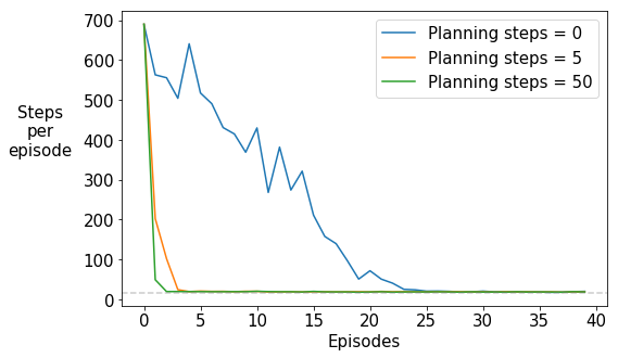
What do you notice?
As the number of planning steps increases, the number of episodes taken to reach the goal decreases rapidly. Remember that the RNG seed was set the same for all the three values of planning steps, resulting in the same number of steps taken to reach the goal in the first episode. Thereafter, the performance improves. The slowest improvement is when there are $n=0$ planning steps, i.e., for the non-planning Q-learning agent, even though the step size parameter was optimized for it. Note that the grey dotted line shows the minimum number of steps required to reach the goal state under the optimal greedy policy.
Experiment(s): Dyna-Q agent in the changing maze environment
Great! Now let us see how Dyna-Q performs on the version of the maze in which a shorter path opens up after 3000 steps. The rest of the transition and reward dynamics remain the same.

Before you proceed, take a moment to think about what you expect to see. Will Dyna-Q find the new, shorter path to the goal? If so, why? If not, why not?
# Do not modify this cell!

def run_experiment_with_state_visitations(env, agent, env_parameters, agent_parameters, exp_parameters, result_file_name):

    # Experiment settings
    num_runs = exp_parameters['num_runs']
    num_max_steps = exp_parameters['num_max_steps']
    planning_steps_all = agent_parameters['planning_steps']

    env_info = {"change_at_n" : env_parameters["change_at_n"]}
    agent_info = {"num_states" : agent_parameters["num_states"],
                  "num_actions" : agent_parameters["num_actions"],
                  "epsilon": agent_parameters["epsilon"],
                  "discount": env_parameters["discount"],
                  "step_size" : agent_parameters["step_size"]}

    state_visits_before_change = np.zeros((len(planning_steps_all), num_runs, 54))  # For saving the number of
    state_visits_after_change = np.zeros((len(planning_steps_all), num_runs, 54))   #     state-visitations
    cum_reward_all = np.zeros((len(planning_steps_all), num_runs, num_max_steps))   # For saving the cumulative reward
    log_data = {'planning_steps_all' : planning_steps_all}

    for idx, planning_steps in enumerate(planning_steps_all):

        print('Planning steps : ', planning_steps)
        os.system('sleep 1')          # to prevent tqdm printing out-of-order before the above print()
        agent_info["planning_steps"] = planning_steps  # We pass the agent the information it needs.

        for run in tqdm(range(num_runs)):

            agent_info['random_seed'] = run
            agent_info['planning_random_seed'] = run

            rl_glue = RLGlue(env, agent)  # Creates a new RLGlue experiment with the env and agent we chose above
            rl_glue.rl_init(agent_info, env_info) # We pass RLGlue what it needs to initialize the agent and environment

            num_steps = 0
            cum_reward = 0

            while num_steps < num_max_steps-1 :

                state, _ = rl_glue.rl_start()  # We start the experiment. We'll be collecting the
                is_terminal = False            # state-visitation counts to visiualize the learned policy
                if num_steps < env_parameters["change_at_n"]:
                    state_visits_before_change[idx][run][state] += 1
                else:
                    state_visits_after_change[idx][run][state] += 1

                while not is_terminal and num_steps < num_max_steps-1 :
                    reward, state, action, is_terminal = rl_glue.rl_step()
                    num_steps += 1
                    cum_reward += reward
                    cum_reward_all[idx][run][num_steps] = cum_reward
                    if num_steps < env_parameters["change_at_n"]:
                        state_visits_before_change[idx][run][state] += 1
                    else:
                        state_visits_after_change[idx][run][state] += 1

    log_data['state_visits_before'] = state_visits_before_change
    log_data['state_visits_after'] = state_visits_after_change
    log_data['cum_reward_all'] = cum_reward_all
    np.save("results/" + result_file_name, log_data)

def plot_cumulative_reward(file_path, item_key, y_key, y_axis_label, legend_prefix, title):

    data_all = np.load(file_path).item()
    data_y_all = data_all[y_key]
    items = data_all[item_key]

    for i, item in enumerate(items):
        plt.plot(np.mean(data_y_all[i], axis=0), label=legend_prefix+str(item))

    plt.axvline(x=3000, linestyle='--', color='grey', alpha=0.4)
    plt.xlabel('Timesteps')
    plt.ylabel(y_axis_label, rotation=0, labelpad=60)
    plt.legend(loc='upper left')
    plt.title(title)
    plt.show()
Did you notice that the environment changes after a fixed number of steps and not episodes?
This is because the environment is separate from the agent, and the environment changes irrespective of the length of each episode (i.e., the number of environmental interactions per episode) that the agent perceives. And hence we are now plotting the data per step or interaction of the agent and the environment, in order to comfortably see the differences in the behaviours of the agents before and after the environment changes.
Okay, now we will first plot the cumulative reward obtained by the agent per interaction with the environment, averaged over 10 runs of the experiment on this changing world.
# Do NOT modify the parameter settings.

# Experiment parameters
experiment_parameters = {
    "num_runs" : 10,                     # The number of times we run the experiment
    "num_max_steps" : 6000,              # The number of steps per experiment
}

# Environment parameters
environment_parameters = {
    "discount": 0.95,
    "change_at_n": 3000
}

# Agent parameters
agent_parameters = {
    "num_states" : 54,
    "num_actions" : 4,
    "epsilon": 0.1,
    "step_size" : 0.125,
    "planning_steps" : [5, 10, 50]      # The list of planning_steps we want to try
}

current_env = ShortcutMazeEnvironment   # The environment
current_agent = DynaQAgent              # The agent

run_experiment_with_state_visitations(current_env, current_agent, environment_parameters, agent_parameters, experiment_parameters, "Dyna-Q_shortcut_steps")
plot_cumulative_reward('results/Dyna-Q_shortcut_steps.npy', 'planning_steps_all', 'cum_reward_all', 'Cumulative\nreward', 'Planning steps = ', 'Dyna-Q : Varying planning_steps')
Planning steps :  5


100%|██████████| 10/10 [00:06<00:00,  1.59it/s]


Planning steps :  10


100%|██████████| 10/10 [00:11<00:00,  1.13s/it]


Planning steps :  50


100%|██████████| 10/10 [00:50<00:00,  5.03s/it]
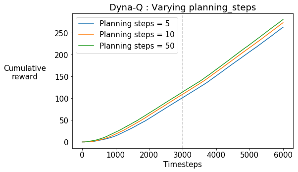
We observe that the slope of the curves is almost constant. If the agent had discovered the shortcut and begun using it, we would expect to see an increase in the slope of the curves towards the later stages of training. This is because the agent can get to the goal state faster and get the positive reward. Note that the timestep at which the shortcut opens up is marked by the grey dotted line.
Note that this trend is constant across the increasing number of planning steps.
Now let’s check the heatmap of the state visitations of the agent with planning_steps=10 during training, before and after the shortcut opens up after 3000 timesteps.
# Do not modify this cell!

def plot_state_visitations(file_path, plot_titles, idx):

    data = np.load(file_path).item()
    data_keys = ["state_visits_before", "state_visits_after"]
    positions = [211,212]
    titles = plot_titles
    wall_ends = [None,-1]

    for i in range(2):

        state_visits = data[data_keys[i]][idx]
        average_state_visits = np.mean(state_visits, axis=0)
        grid_state_visits = np.rot90(average_state_visits.reshape((6,9)).T)
        grid_state_visits[2,1:wall_ends[i]] = np.nan # walls
        #print(average_state_visits.reshape((6,9)))
        plt.subplot(positions[i])
        plt.pcolormesh(grid_state_visits, edgecolors='gray', linewidth=1, cmap='viridis')
        plt.text(3+0.5, 0+0.5, 'S', horizontalalignment='center', verticalalignment='center')
        plt.text(8+0.5, 5+0.5, 'G', horizontalalignment='center', verticalalignment='center')
        plt.title(titles[i])
        plt.axis('off')
        cm = plt.get_cmap()
        cm.set_bad('gray')

    plt.subplots_adjust(bottom=0.0, right=0.7, top=1.0)
    cax = plt.axes([1., 0.0, 0.075, 1.])
    cbar = plt.colorbar(cax=cax)
    plt.show()
# Do not modify this cell!

plot_state_visitations("results/Dyna-Q_shortcut_steps.npy", ['Dyna-Q : State visitations before the env changes', 'Dyna-Q : State visitations after the env changes'], 1)
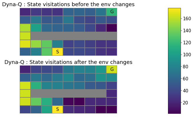
What do you observe?
The state visitation map looks almost the same before and after the shortcut opens. This means that the Dyna-Q agent hasn’t quite discovered and started exploiting the new shortcut.
Now let’s try increasing the exploration parameter $\epsilon$ to see if it helps the Dyna-Q agent discover the shortcut.
# Do not modify this cell!

def run_experiment_only_cumulative_reward(env, agent, env_parameters, agent_parameters, exp_parameters):

    # Experiment settings
    num_runs = exp_parameters['num_runs']
    num_max_steps = exp_parameters['num_max_steps']
    epsilons = agent_parameters['epsilons']

    env_info = {"change_at_n" : env_parameters["change_at_n"]}
    agent_info = {"num_states" : agent_parameters["num_states"],
                  "num_actions" : agent_parameters["num_actions"],
                  "planning_steps": agent_parameters["planning_steps"],
                  "discount": env_parameters["discount"],
                  "step_size" : agent_parameters["step_size"]}

    log_data = {'epsilons' : epsilons}
    cum_reward_all = np.zeros((len(epsilons), num_runs, num_max_steps))

    for eps_idx, epsilon in enumerate(epsilons):

        print('Agent : Dyna-Q, epsilon : %f' % epsilon)
        os.system('sleep 1')          # to prevent tqdm printing out-of-order before the above print()
        agent_info["epsilon"] = epsilon

        for run in tqdm(range(num_runs)):

            agent_info['random_seed'] = run
            agent_info['planning_random_seed'] = run

            rl_glue = RLGlue(env, agent)  # Creates a new RLGlue experiment with the env and agent we chose above
            rl_glue.rl_init(agent_info, env_info) # We pass RLGlue what it needs to initialize the agent and environment

            num_steps = 0
            cum_reward = 0

            while num_steps < num_max_steps-1 :

                rl_glue.rl_start()  # We start the experiment
                is_terminal = False

                while not is_terminal and num_steps < num_max_steps-1 :
                    reward, _, action, is_terminal = rl_glue.rl_step()  # The environment and agent take a step and return
                    # the reward, and action taken.
                    num_steps += 1
                    cum_reward += reward
                    cum_reward_all[eps_idx][run][num_steps] = cum_reward

    log_data['cum_reward_all'] = cum_reward_all
    np.save("results/Dyna-Q_epsilons", log_data)
# Do NOT modify the parameter settings.

# Experiment parameters
experiment_parameters = {
    "num_runs" : 30,                     # The number of times we run the experiment
    "num_max_steps" : 6000,              # The number of steps per experiment
}

# Environment parameters
environment_parameters = {
    "discount": 0.95,
    "change_at_n": 3000
}

# Agent parameters
agent_parameters = {
    "num_states" : 54,
    "num_actions" : 4,
    "step_size" : 0.125,
    "planning_steps" : 10,
    "epsilons": [0.1, 0.2, 0.4, 0.8]    # The list of epsilons we want to try
}

current_env = ShortcutMazeEnvironment   # The environment
current_agent = DynaQAgent              # The agent

run_experiment_only_cumulative_reward(current_env, current_agent, environment_parameters, agent_parameters, experiment_parameters)
plot_cumulative_reward('results/Dyna-Q_epsilons.npy', 'epsilons', 'cum_reward_all', 'Cumulative\nreward', r'$\epsilon$ = ', r'Dyna-Q : Varying $\epsilon$')
Agent : Dyna-Q, epsilon : 0.100000


100%|██████████| 30/30 [00:33<00:00,  1.13s/it]


Agent : Dyna-Q, epsilon : 0.200000


100%|██████████| 30/30 [00:33<00:00,  1.13s/it]


Agent : Dyna-Q, epsilon : 0.400000


100%|██████████| 30/30 [00:33<00:00,  1.12s/it]


Agent : Dyna-Q, epsilon : 0.800000


100%|██████████| 30/30 [00:33<00:00,  1.11s/it]
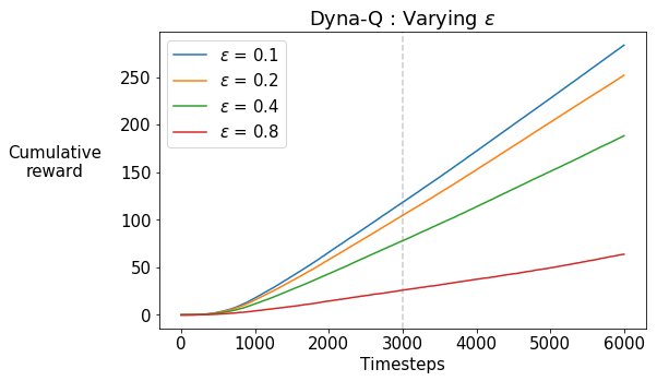
What do you observe?
Increasing the exploration via the $\epsilon$-greedy strategy does not seem to be helping. In fact, the agent’s cumulative reward decreases because it is spending more and more time trying out the exploratory actions.
Can we do better…?
Section 2: Dyna-Q+
The motivation behind Dyna-Q+ is to give a bonus reward for actions that haven’t been tried for a long time, since there is a greater chance that the dynamics for that actions might have changed.
In particular, if the modeled reward for a transition is $r$, and the transition has not been tried in $\tau(s,a)$ time steps, then planning updates are done as if that transition produced a reward of $r + \kappa \sqrt{ \tau(s,a)}$, for some small $\kappa$.
Let’s implement that!
Based on your DynaQAgent, create a new class DynaQPlusAgent to implement the aforementioned exploration heuristic. Additionally :
- actions that had never been tried before from a state should now be allowed to be considered in the planning step,
- and the initial model for such actions is that they lead back to the same state with a reward of zero.
At this point, you might want to refer to the video lectures and Section 8.3 of the RL textbook for a refresher on Dyna-Q+.
As usual, let’s break this down in pieces and do it one-by-one.
First of all, check out the agent_init method below. In particular, pay attention to the attributes which are new to DynaQPlusAgent– state-visitation counts $\tau$ and the scaling parameter $\kappa$ – because you shall be using them later.
# Do not modify this cell!

class DynaQPlusAgent(BaseAgent):

    def agent_init(self, agent_info):
        """Setup for the agent called when the experiment first starts.

        Args:
            agent_init_info (dict), the parameters used to initialize the agent. The dictionary contains:
            {
                num_states (int): The number of states,
                num_actions (int): The number of actions,
                epsilon (float): The parameter for epsilon-greedy exploration,
                step_size (float): The step-size,
                discount (float): The discount factor,
                planning_steps (int): The number of planning steps per environmental interaction
                kappa (float): The scaling factor for the reward bonus

                random_seed (int): the seed for the RNG used in epsilon-greedy
                planning_random_seed (int): the seed for the RNG used in the planner
            }
        """

        # First, we get the relevant information from agent_info
        # Note: we use np.random.RandomState(seed) to set the two different RNGs
        # for the planner and the rest of the code
        try:
            self.num_states = agent_info["num_states"]
            self.num_actions = agent_info["num_actions"]
        except:
            print("You need to pass both 'num_states' and 'num_actions' \
                   in agent_info to initialize the action-value table")
        self.gamma = agent_info.get("discount", 0.95)
        self.step_size = agent_info.get("step_size", 0.1)
        self.epsilon = agent_info.get("epsilon", 0.1)
        self.planning_steps = agent_info.get("planning_steps", 10)
        self.kappa = agent_info.get("kappa", 0.001)

        self.rand_generator = np.random.RandomState(agent_info.get('random_seed', 42))
        self.planning_rand_generator = np.random.RandomState(agent_info.get('planning_random_seed', 42))

        # Next, we initialize the attributes required by the agent, e.g., q_values, model, tau, etc.
        # The visitation-counts can be stored as a table as well, like the action values
        self.q_values = np.zeros((self.num_states, self.num_actions))
        self.tau = np.zeros((self.num_states, self.num_actions))
        self.actions = list(range(self.num_actions))
        self.past_action = -1
        self.past_state = -1
        self.model = {}
Now first up, implement the update_model method. Note that this is different from Dyna-Q in the aforementioned way.
%%add_to DynaQPlusAgent

# [GRADED]

def update_model(self, past_state, past_action, state, reward):
    """updates the model

    Args:
        past_state  (int): s
        past_action (int): a
        state       (int): s'
        reward      (int): r
    Returns:
        Nothing
    """

    # Recall that when adding a state-action to the model, if the agent is visiting the state
    #    for the first time, then the remaining actions need to be added to the model as well
    #    with zero reward and a transition into itself. Something like:
    ##   for action in self.actions:
    ##       if action != past_action:
    ##           self.model[past_state][action] = (past_state, 0)
    #
    # Note: do *not* update the visitation-counts here. We will do that in `agent_step`.
    #
    # (3 lines)

    if past_state not in self.model:
        self.model[past_state] = {past_action : (state, reward)}
        ### START CODE HERE ###
        for action in self.actions:
            if action != past_action:
                self.model[past_state][action] = (past_state, 0)
        ### END CODE HERE ###
    else:
        self.model[past_state][past_action] = (state, reward)
Test update_model()
# Do not modify this cell!

## Test code for update_model() ##

actions = []
agent_info = {"num_actions": 4,
              "num_states": 3,
              "epsilon": 0.1,
              "step_size": 0.1,
              "discount": 1.0,
              "random_seed": 0,
              "planning_random_seed": 0}
test_agent = DynaQPlusAgent()
test_agent.agent_init(agent_info)
test_agent.update_model(0,2,0,1)
test_agent.update_model(2,0,1,1)
test_agent.update_model(0,3,1,2)
test_agent.tau[0][0] += 1
print("Model: \n", test_agent.model)
Model:
 {0: {2: (0, 1), 0: (0, 0), 1: (0, 0), 3: (1, 2)}, 2: {0: (1, 1), 1: (2, 0), 2: (2, 0), 3: (2, 0)}}
Expected output:
Model:
 {0: {2: (0, 1), 0: (0, 0), 1: (0, 0), 3: (1, 2)}, 2: {0: (1, 1), 1: (2, 0), 2: (2, 0), 3: (2, 0)}}
Note that the actions that were not taken from a state are also added to the model, with a loop back into the same state with a reward of 0.
Next, you will implement the planning_step() method. This will be very similar to the one you implemented in DynaQAgent, but here you will be adding the exploration bonus to the reward in the simulated transition.
%%add_to DynaQPlusAgent

# [GRADED]

def planning_step(self):
    """performs planning, i.e. indirect RL.

    Args:
        None
    Returns:
        Nothing
    """

    # The indirect RL step:
    # - Choose a state and action from the set of experiences that are stored in the model. (~2 lines)
    # - Query the model with this state-action pair for the predicted next state and reward.(~1 line)
    # - **Add the bonus to the reward** (~1 line)
    # - Update the action values with this simulated experience.                            (2~4 lines)
    # - Repeat for the required number of planning steps.
    #
    # Note that the update equation is different for terminal and non-terminal transitions.
    # To differentiate between a terminal and a non-terminal next state, assume that the model stores
    # the terminal state as a dummy state like -1
    #
    # Important: remember you have a random number generator 'planning_rand_generator' as
    #     a part of the class which you need to use as self.planning_rand_generator.choice()
    #     For the sake of reproducibility and grading, *do not* use anything else like
    #     np.random.choice() for performing search control.

    ### START CODE HERE ###
    for i in range(self.planning_steps):
        past_state = self.planning_rand_generator.choice(list(self.model.keys()))
        past_action = self.planning_rand_generator.choice(list(self.model[past_state].keys()))
        next_state, reward = self.model[past_state][past_action]
        reward += self.kappa * np.sqrt(self.tau[past_state, past_action])

        if next_state == -1:
            q_max = 0
        else:
            q_max = np.max(self.q_values[next_state])

        self.q_values[past_state, past_action] += self.step_size * (reward + self.gamma * q_max
                                                                    - self.q_values[past_state, past_action])
    ### END CODE HERE ###
Test planning_step()
# Do not modify this cell!

## Test code for planning_step() ##

actions = []
agent_info = {"num_actions": 4,
              "num_states": 3,
              "epsilon": 0.1,
              "step_size": 0.1,
              "discount": 1.0,
              "kappa": 0.001,
              "planning_steps": 4,
              "random_seed": 0,
              "planning_random_seed": 1}
test_agent = DynaQPlusAgent()
test_agent.agent_init(agent_info)
test_agent.update_model(0,1,-1,1)
test_agent.tau += 1; test_agent.tau[0][1] = 0
test_agent.update_model(0,2,1,1)
test_agent.tau += 1; test_agent.tau[0][2] = 0    # Note that these counts are manually updated
test_agent.update_model(2,0,1,1)                 #     as we'll code them in `agent_step'
test_agent.tau += 1; test_agent.tau[2][0] = 0    #     which hasn't been implemented yet.

test_agent.planning_step()

print("Model: \n", test_agent.model)
print("Action-value estimates: \n", test_agent.q_values)
Model:
 {0: {1: (-1, 1), 0: (0, 0), 2: (1, 1), 3: (0, 0)}, 2: {0: (1, 1), 1: (2, 0), 2: (2, 0), 3: (2, 0)}}
Action-value estimates:
 [[0.         0.10014142 0.         0.        ]
 [0.         0.         0.         0.        ]
 [0.         0.00036373 0.         0.00017321]]
Expected output:
Model:
 {0: {1: (-1, 1), 0: (0, 0), 2: (1, 1), 3: (0, 0)}, 2: {0: (1, 1), 1: (2, 0), 2: (2, 0), 3: (2, 0)}}
Action-value estimates:
 [[0.         0.10014142 0.         0.        ]
 [0.         0.         0.         0.        ]
 [0.         0.00036373 0.         0.00017321]]
Again, before you move on to implement the rest of the agent methods, here are the couple of helper functions that you’ve used in the previous assessments for choosing an action using an $\epsilon$-greedy policy.
%%add_to DynaQPlusAgent

# Do not modify this cell!

def argmax(self, q_values):
    """argmax with random tie-breaking
    Args:
        q_values (Numpy array): the array of action values
    Returns:
        action (int): an action with the highest value
    """
    top = float("-inf")
    ties = []

    for i in range(len(q_values)):
        if q_values[i] > top:
            top = q_values[i]
            ties = []

        if q_values[i] == top:
            ties.append(i)

    return self.rand_generator.choice(ties)

def choose_action_egreedy(self, state):
    """returns an action using an epsilon-greedy policy w.r.t. the current action-value function.

    Important: assume you have a random number generator 'rand_generator' as a part of the class
                which you can use as self.rand_generator.choice() or self.rand_generator.rand()

    Args:
        state (List): coordinates of the agent (two elements)
    Returns:
        The action taken w.r.t. the aforementioned epsilon-greedy policy
    """

    if self.rand_generator.rand() < self.epsilon:
        action = self.rand_generator.choice(self.actions)
    else:
        values = self.q_values[state]
        action = self.argmax(values)

    return action
Now implement the rest of the agent-related methods, namely agent_start, agent_step, and agent_end. Again, these will be very similar to the ones in the DynaQAgent, but you will have to think of a way to update the counts since the last visit.
%%add_to DynaQPlusAgent

# [GRADED]

def agent_start(self, state):
    """The first method called when the experiment starts, called after
    the environment starts.
    Args:
        state (Numpy array): the state from the
            environment's env_start function.
    Returns:
        (int) The first action the agent takes.
    """

    # given the state, select the action using self.choose_action_egreedy(),
    # and save current state and action (~2 lines)
    ### self.past_state = ?
    ### self.past_action = ?
    # Note that the last-visit counts are not updated here.

    ### START CODE HERE ###
    action = self.choose_action_egreedy(state)

    self.past_state = state
    self.past_action = action
    ### END CODE HERE ###

    return self.past_action

def agent_step(self, reward, state):
    """A step taken by the agent.
    Args:
        reward (float): the reward received for taking the last action taken
        state (Numpy array): the state from the
            environment's step based on where the agent ended up after the
            last step
    Returns:
        (int) The action the agent is taking.
    """

    # Update the last-visited counts (~2 lines)
    # - Direct-RL step (1~3 lines)
    # - Model Update step (~1 line)
    # - `planning_step` (~1 line)
    # - Action Selection step (~1 line)
    # Save the current state and action before returning the action to be performed. (~2 lines)

    ### START CODE HERE ###
    # Tau Update step
    self.tau += 1
    self.tau[self.past_state, self.past_action] = 0
    # Direct-RL step
    q_max = np.max(self.q_values[state])
    self.q_values[self.past_state, self.past_action] += self.step_size * (reward + self.gamma * q_max
                                                                - self.q_values[self.past_state, self.past_action])
    # Model Update step
    self.update_model(self.past_state, self.past_action, state, reward)
    # Planning
    self.planning_step()
    # Choose Action
    action = self.choose_action_egreedy(state)
    # Save the current state and action
    self.past_state = state
    self.past_action = action
    ### END CODE HERE ###

    return self.past_action

def agent_end(self, reward):
    """Called when the agent terminates.
    Args:
        reward (float): the reward the agent received for entering the
            terminal state.
    """
    # Again, add the same components you added in agent_step to augment Dyna-Q into Dyna-Q+

    ### START CODE HERE ###
    # Tau Update step
    self.tau += 1
    self.tau[self.past_state, self.past_action] = 0
    # Direct-RL step
    self.q_values[self.past_state, self.past_action] += self.step_size * (reward
                                                                          - self.q_values[self.past_state, self.past_action])
    # Model Update step
    self.update_model(self.past_state, self.past_action, -1, reward)
    # Planning
    self.planning_step()
    ### END CODE HERE ###
Let’s test these methods one-by-one.
Test agent_start()
# Do not modify this cell!

## Test code for agent_start() ##

agent_info = {"num_actions": 4,
              "num_states": 3,
              "epsilon": 0.1,
              "step_size": 0.1,
              "discount": 1.0,
              "kappa": 0.001,
              "random_seed": 0,
              "planning_random_seed": 0}
test_agent = DynaQPlusAgent()
test_agent.agent_init(agent_info)
action = test_agent.agent_start(0) # state
print("Action:", action)
print("Timesteps since last visit: \n", test_agent.tau)
print("Action-value estimates: \n", test_agent.q_values)
print("Model: \n", test_agent.model)
Action: 1
Timesteps since last visit:
 [[0. 0. 0. 0.]
 [0. 0. 0. 0.]
 [0. 0. 0. 0.]]
Action-value estimates:
 [[0. 0. 0. 0.]
 [0. 0. 0. 0.]
 [0. 0. 0. 0.]]
Model:
 {}
Expected output:
Action: 1
Timesteps since last visit:
 [[0. 0. 0. 0.]
 [0. 0. 0. 0.]
 [0. 0. 0. 0.]]
Action-value estimates:
 [[0. 0. 0. 0.]
 [0. 0. 0. 0.]
 [0. 0. 0. 0.]]
Model:
 {}
Remember the last-visit counts are not updated in agent_start().
Test agent_step()
# Do not modify this cell!

## Test code for agent_step() ##

agent_info = {"num_actions": 4,
              "num_states": 3,
              "epsilon": 0.1,
              "step_size": 0.1,
              "discount": 1.0,
              "kappa": 0.001,
              "planning_steps": 4,
              "random_seed": 0,
              "planning_random_seed": 0}
test_agent = DynaQPlusAgent()
test_agent.agent_init(agent_info)
actions = []
actions.append(test_agent.agent_start(0))    # state
actions.append(test_agent.agent_step(1,2))   # (reward, state)
actions.append(test_agent.agent_step(0,1))   # (reward, state)
print("Actions:", actions)
print("Timesteps since last visit: \n", test_agent.tau)
print("Action-value estimates: \n", test_agent.q_values)
print("Model: \n", test_agent.model)
Actions: [1, 3, 1]
Timesteps since last visit:
 [[2. 1. 2. 2.]
 [2. 2. 2. 2.]
 [2. 2. 2. 0.]]
Action-value estimates:
 [[1.91000000e-02 2.71000000e-01 0.00000000e+00 1.91000000e-02]
 [0.00000000e+00 0.00000000e+00 0.00000000e+00 0.00000000e+00]
 [0.00000000e+00 1.83847763e-04 4.24264069e-04 0.00000000e+00]]
Model:
 {0: {1: (2, 1), 0: (0, 0), 2: (0, 0), 3: (0, 0)}, 2: {3: (1, 0), 0: (2, 0), 1: (2, 0), 2: (2, 0)}}
Expected output:
Actions: [1, 3, 1]
Timesteps since last visit:
 [[2. 1. 2. 2.]
 [2. 2. 2. 2.]
 [2. 2. 2. 0.]]
Action-value estimates:
 [[1.91000000e-02 2.71000000e-01 0.00000000e+00 1.91000000e-02]
 [0.00000000e+00 0.00000000e+00 0.00000000e+00 0.00000000e+00]
 [0.00000000e+00 1.83847763e-04 4.24264069e-04 0.00000000e+00]]
Model:
 {0: {1: (2, 1), 0: (0, 0), 2: (0, 0), 3: (0, 0)}, 2: {3: (1, 0), 0: (2, 0), 1: (2, 0), 2: (2, 0)}}
Test agent_end()
# Do not modify this cell!

## Test code for agent_end() ##

agent_info = {"num_actions": 4,
              "num_states": 3,
              "epsilon": 0.1,
              "step_size": 0.1,
              "discount": 1.0,
              "kappa": 0.001,
              "planning_steps": 4,
              "random_seed": 0,
              "planning_random_seed": 0}
test_agent = DynaQPlusAgent()
test_agent.agent_init(agent_info)
actions = []
actions.append(test_agent.agent_start(0))
actions.append(test_agent.agent_step(1,2))
actions.append(test_agent.agent_step(0,1))
test_agent.agent_end(1)
print("Actions:", actions)
print("Timesteps since last visit: \n", test_agent.tau)
print("Action-value estimates: \n", test_agent.q_values)
print("Model: \n", test_agent.model)
Actions: [1, 3, 1]
Timesteps since last visit:
 [[3. 2. 3. 3.]
 [3. 0. 3. 3.]
 [3. 3. 3. 1.]]
Action-value estimates:
 [[1.91000000e-02 3.44083848e-01 0.00000000e+00 4.44632051e-02]
 [1.91732051e-02 1.90000000e-01 0.00000000e+00 0.00000000e+00]
 [0.00000000e+00 1.83847763e-04 4.24264069e-04 0.00000000e+00]]
Model:
 {0: {1: (2, 1), 0: (0, 0), 2: (0, 0), 3: (0, 0)}, 2: {3: (1, 0), 0: (2, 0), 1: (2, 0), 2: (2, 0)}, 1: {1: (-1, 1), 0: (1, 0), 2: (1, 0), 3: (1, 0)}}
Expected output:
Actions: [1, 3, 1]
Timesteps since last visit:
 [[3. 2. 3. 3.]
 [3. 0. 3. 3.]
 [3. 3. 3. 1.]]
Action-value estimates:
 [[1.91000000e-02 3.44083848e-01 0.00000000e+00 4.44632051e-02]
 [1.91732051e-02 1.90000000e-01 0.00000000e+00 0.00000000e+00]
 [0.00000000e+00 1.83847763e-04 4.24264069e-04 0.00000000e+00]]
Model:
 {0: {1: (2, 1), 0: (0, 0), 2: (0, 0), 3: (0, 0)}, 2: {3: (1, 0), 0: (2, 0), 1: (2, 0), 2: (2, 0)}, 1: {1: (-1, 1), 0: (1, 0), 2: (1, 0), 3: (1, 0)}}
Experiment: Dyna-Q+ agent in the changing environment
Okay, now we’re ready to test our Dyna-Q+ agent on the Shortcut Maze. As usual, we will average the results over 30 independent runs of the experiment.
# Do NOT modify the parameter settings.

# Experiment parameters
experiment_parameters = {
    "num_runs" : 30,                     # The number of times we run the experiment
    "num_max_steps" : 6000,              # The number of steps per experiment
}

# Environment parameters
environment_parameters = {
    "discount": 0.95,
    "change_at_n": 3000
}

# Agent parameters
agent_parameters = {
    "num_states" : 54,
    "num_actions" : 4,
    "epsilon": 0.1,
    "step_size" : 0.5,
    "planning_steps" : [50]
}

current_env = ShortcutMazeEnvironment   # The environment
current_agent = DynaQPlusAgent          # The agent

run_experiment_with_state_visitations(current_env, current_agent, environment_parameters, agent_parameters, experiment_parameters, "Dyna-Q+")
shutil.make_archive('results', 'zip', 'results');
Planning steps :  50


100%|██████████| 30/30 [02:55<00:00,  5.86s/it]
Let’s compare the Dyna-Q and Dyna-Q+ agents with planning_steps=50 each.
# Do not modify this cell!

def plot_cumulative_reward_comparison(file_name_dynaq, file_name_dynaqplus):

    cum_reward_q = np.load(file_name_dynaq).item()['cum_reward_all'][2]
    cum_reward_qPlus = np.load(file_name_dynaqplus).item()['cum_reward_all'][0]

    plt.plot(np.mean(cum_reward_qPlus, axis=0), label='Dyna-Q+')
    plt.plot(np.mean(cum_reward_q, axis=0), label='Dyna-Q')

    plt.axvline(x=3000, linestyle='--', color='grey', alpha=0.4)
    plt.xlabel('Timesteps')
    plt.ylabel('Cumulative\nreward', rotation=0, labelpad=60)
    plt.legend(loc='upper left')
    plt.title('Average performance of Dyna-Q and Dyna-Q+ agents in the Shortcut Maze\n')
    plt.show()
# Do not modify this cell!

plot_cumulative_reward_comparison('results/Dyna-Q_shortcut_steps.npy', 'results/Dyna-Q+.npy')
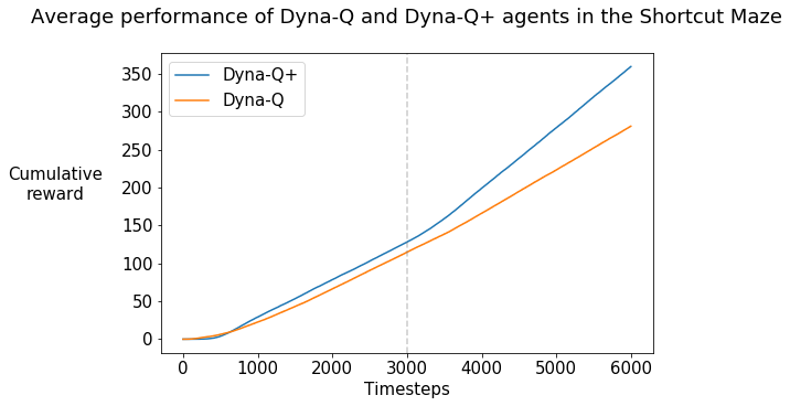
What do you observe? (For reference, your graph should look like Figure 8.5 in Chapter 8 of the RL textbook)
The slope of the curve increases for the Dyna-Q+ curve shortly after the shortcut opens up after 3000 steps, which indicates that the rate of receiving the positive reward increases. This implies that the Dyna-Q+ agent finds the shorter path to the goal.
To verify this, let us plot the state-visitations of the Dyna-Q+ agent before and after the shortcut opens up.
# Do not modify this cell!

plot_state_visitations("results/Dyna-Q+.npy", ['Dyna-Q+ : State visitations before the env changes', 'Dyna-Q+ : State visitations after the env changes'], 0)
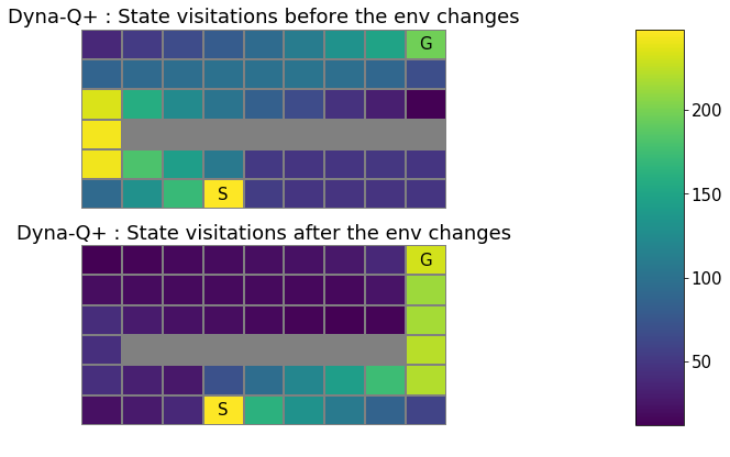
What do you observe?
Before the shortcut opens up, like Dyna-Q, the Dyna-Q+ agent finds the sole, long path to the goal. But because the Dyna-Q+ agent keeps exploring, it succeeds in discovering the shortcut once it opens up, which leads to the goal faster. So the bonus reward heuristic is effective in helping the agent explore and find changes in the environment without degrading the performance.
Wrapping Up
Congratulations! You have:
- implemented Dyna-Q, a model-based approach to RL;
- implemented Dyna-Q+, a variant of Dyna-Q with an exploration bonus that encourages exploration;
- conducted scientific experiments to empirically validate the exploration/exploitation dilemma in the planning context on an environment that changes with time.
Some points to ponder about:
- At what cost does Dyna-Q+ improve over Dyna-Q?
- In general, what is the trade-off of using model-based methods like Dyna-Q over model-free methods like Q-learning?
Note: Apart from using the ‘Submit’ button in the notebook, you have to submit an additional zip file containing the ‘npy’ files that were generated from running the experiment cells. To do so:
- Generate the zip file by running the experiment cells in the notebook. On the top of the notebook, navigate to ‘File->Open’ to open the directory view of this assignment. Select “results.zip” and click on “Download”. Alternatively, you can download just the results folder and run “zip -jr results.zip results/” (The flag ‘j’ is required by the grader!).
- Go to the “My submission” tab and click on “+ Create submission”.
- Click on “C2M4 Data-file Grader” and upload your
results.zip.
This accounts for 50% of the marks, so don’t forget to do so!