Welcome to your final course project on RL in Finance. In this project you will:
- Explore and estimate an IRL-based model of market returns that is based on IRL of a market-optimal portfolio
- Investigate the role and impact of choices of different signals on model estimation and trading strategies
- Compare simple IRL-based and UL-based trading strategies
Instructions for project structure and grading principles :
-
This is a project that will be graded based on a peer-to-peer review. The project consists of four parts. The maximum score for each part is 10, so that maximum score you can give your peers (and they can give you) is 40. The parts are as follows (more detailed instructions are in specific cells below):
-
Part 1: Complete the model estimation for the DJI portfolio of 30 stocks, and simple signals such as simple moving averages constructed below (Max 10 point).
-
Part 2: Propose other signals and investigate the dynamics for market caps obtained with alternative signals. Present your conclusions and observations. (Max 10 point).
-
Part 3: Can you repeat your analysis for the S&P portfolio? You will have to build a data file, build signals, and repeat the model estimation process with your new dataset (Max 10 points).
-
Part 4 : Show me something else. This part is optional. Come up with your own idea of an interesting analysis. For example, you can build a strategy using an optimal market-implied policy estimated from this model, and compare it with PCA and absorption ratio strategies that we built in Course 2. (Max 10 points).
**Instructions for formatting your notebook and packages use can use **
-
Use one or more cells of the notebook for each section of the project. Each section is marked by a header cell below. Insert your cells between them without changing the sequence.
-
Think of an optimal presentation of your results and conclusions. Think of how hard or easy it will be for your fellow students to follow your logic and presentation. When you are grading others, you can add or subtract point for the quality of presentation.
-
You will be using Python 3 in this project. Using TensorFlow is encouraged but is not strictly necessary, you can use optimization algorithms available in scipy or scikit-learn packages. If you use any non-standard packages, you should state all neccessary additional imports (or instructions how to install any additional modules you use in a top cell of your notebook. If you create a new portfolio for parts 3 and 4 in the project, make your code for creating your dataset replicable as well, so that your grader can reproduce your code locally on his/her machine.
-
Try to write a clean code that can be followed by your peer reviewer. When you are the reviewer, you can add or subtract point for the quality of code.
After completing this project you will:
- Get experience with building and estimation of your first IRL based model of market dynamics, and learn how this IRL approach extends the famous Black-Litterman model (see F. Black and R. Litterman, “Global Portfolio Optimization”, Financial Analyst Journal, Sept-Oct. 1992, 28-43, and D. Bertsimas, V. Gupta, and I.Ch. Paschalidis, “Inverse Optimization: A New Perspective on the Black-Litterman Model”, Operations Research, Vol.60, No.6, pp. 1389-1403 (2012), I.Halperin and I. Feldshteyn “Market Self-Learning of Signals, Impact and Optimal Trading: Invisible Hand Inference with Free Energy”, https://papers.ssrn.com/sol3/papers.cfm?abstract_id=3174498.).
- Know how to enhance a market-optimal portfolio policy by using your private signals.
- Be able to implement trading strategies based on this method.
Let’s get started!
The IRL-based model of stock returns
In Week 4 lectures of our course we found that optimal investment policy in the problem of inverse portfolio optimization is a Gaussian policy
\[\pi_{\theta}({\bf a}_t |{\bf y}_t ) = \mathcal{N}\left({\bf a}_t | \bf{A}_0 + \bf{A}_1 {\bf y}_t, \Sigma_p \right)\]Here \({\bf y}_t\) is a vector of dollar position in the portfolio, and \(\bf{A}_0\), \(\bf{A}_1\) and \(\Sigma_p\) are parameters defining a Gaussian policy.
We said in the lecture that such Gaussian policy is found for both cases of a single investor and a market portfolio. We also sketched a numerical scheme that can iteratively compute coefficients \(\bf{A}_0\), \(\bf{A}_1\) and \(\Sigma_p\) using a combination of a RL algorithm called G-learning and a trajectory optimization algorithm.
In this project, you will explore implications and estimation of this IRL-based model for the most interesting case - the market portfolio. It turns out that for this case, the model can be estimated in an easier way using a conventional Maximum Likelihood approach. To this end, we will re-formulate the model for this particular case in three easy steps.
Recall that for a vector of \(N\) stocks, we introduced a size \(2 N\)-action vector \({\bf a}_t = [{\bf u}_t^{(+)}, {\bf u}_t^{(-)}]\), so that an action \({\bf u}_t\) was defined as a difference of two non-negative numbers \({\bf u}_t = {\bf u}_t^{(+)} - {\bf u}_t^{(-)} = [{\bf 1}, - {\bf 1}] {\bf a}_t \equiv {\bf 1}_{-1}^{T} {\bf a}_t\).
Therefore, the joint distribution of \({\bf a}_t = [{\bf u}_t^{(+)}, {\bf u}_t^{(-)} ]\) is given by our Gaussian policy \(\pi_{\theta}({\bf a}_t |{\bf y}_t )\). This means that the distribution of \({\bf u}_t = {\bf u}_t^{(+)} - {\bf u}_t^{(-)}\) is also Gaussian. Let us write it therefore as follows:
\[\pi_{\theta}({\bf u}_t |{\bf y}_t ) = \mathcal{N}\left({\bf u}_t | \bf{U}_0 + \bf{U}_1 {\bf y}_t, \Sigma_u \right)\]Here \(\bf{U}_0 = {\bf 1}_{-1}^{T} \bf{A}_0\) and \(\bf{U}_1 = {\bf 1}_{-1}^{T} \bf{A}_1\).
This means that \({\bf u}_t\) is a Gaussian random variable that we can write as follows:
\[{\bf u}_t = \bf{U}_0 + \bf{U}_1 {\bf y}_t + \varepsilon_t^{(u)} = \bf{U}_0 + \bf{U}_1^{(x)} {\bf x}_t + \bf{U}_1^{(z)} {\bf z}_t + \varepsilon_t^{(u)}\]where \(\varepsilon_t^{(u)} \sim \mathcal{N}(0,\Sigma_u)\) is a Gaussian random noise.
The most important feature of this expression that we need going forward is is linear dependence on the state \({\bf x}_t\). This is the only result that we will use in order to construct a simple dynamic market model resulting from our IRL model. We use a deterministic limit of this equation, where in addition we set \(\bf{U}_0 = \bf{U}_1^{(z)} = 0\), and replace \(\bf{U}_1^{(x)} \rightarrow \phi\) to simplify the notation. We thus obtain a simple deterministic policy
\[\label{determ_u} {\bf u}_t = \phi {\bf x}_t\]Next, let us recall the state equation and return equation (where we reinstate a time step \(\Delta t\), and \(\circ\) stands for an element-wise (Hadamard) product):
\(X_{t+ \Delta t} = (1 + r_t \Delta t) \circ ( X_t + u_t \Delta t)\) \(r_t = r_f + {\bf w} {\bf z}_t - \mu u_t + \frac{\sigma}{ \sqrt{ \Delta t}} \varepsilon_t\) where \(r_f\) is a risk-free rate, \(\Delta t\) is a time step, \({\bf z}_t\) is a vector of predictors with weights \({\bf w}\), \(\mu\) is a market impact parameter with a linear impact specification, and \(\varepsilon_t \sim \mathcal{N} (\cdot| 0, 1)\) is a white noise residual.
Eliminating \(u_t\) from these expressions and simplifying, we obtain \(\Delta X_t = \mu \phi ( 1 + \phi \Delta t) \circ X_t \circ \left( \frac{r_f (1 + \phi \Delta t) + \phi}{ \mu \phi (1+ \phi \Delta t )} - X_t \right) \Delta t + ( 1 + \phi \Delta t) X_t \circ \left[ {\bf w} {\bf z}_t \Delta t + \sigma \sqrt{ \Delta t} \varepsilon_t \right]\)
Finally, assuming that \(\phi \Delta t \ll 1\) and taking the continuous-time limit \(\Delta t \rightarrow dt\), we obtain
\(d X_t = \kappa \circ X_t \circ \left( \frac{\theta}{\kappa} - X_t \right) dt + X_t \circ \left[ {\bf w} {\bf z}_t \, dt + \sigma d W_t \right]\) where \(\kappa = \mu \phi\), \(\theta = r_f + \phi\), and \(W_t\) is a standard Brownian motion.
Please note that this equation describes dynamics with a quadratic mean reversion. It is quite different from models with linear mean reversion such as the Ornstein-Uhlenbeck (OU) process.
Without signals \({\bf z}_t\), this process is known in the literature as a Geometric Mean Reversion (GMR) process. It has been used (for a one-dimensional setting) by Dixit and Pyndick (“ Investment Under Uncertainty”, Princeton 1994), and investigated (also for 1D) by Ewald and Yang (“Geometric Mean Reversion: Formulas for the Equilibrium Density and Analytic Moment Matching”, {\it University of St. Andrews Economics Preprints}, 2007). We have found that such dynamics (in a multi-variate setting) can also be obtained for market caps (or equivalently for stock prices, so long as the number of shares is held fixed) using Inverse Reinforcement Learning!
(For more details, see I. Halperin and I. Feldshteyn, “Market Self-Learning of Signals, Impact and Optimal Trading: Invisible Hand Inference with Free Energy. (or, How We Learned to Stop Worrying and Love Bounded Rationality)”, https://papers.ssrn.com/sol3/papers.cfm?abstract_id=3174498)
import pandas as pd
import numpy as np
import tensorflow as tf

import matplotlib.pyplot as plt
from datetime import datetime
# read the data to a Dataframe
df_cap = pd.read_csv('dja_cap.csv')
# add dates
dates = pd.bdate_range(start='2010-01-04', end=None, periods=df_cap.shape[0], freq='B')
df_cap['date'] = dates

df_cap.set_index('date',inplace=True)
df_cap.head()
| AAPL | AXP | BA | CAT | CSCO | CVX | DIS | DWDP | GE | GS | ... | NKE | PFE | PG | TRV | UNH | UTX | V | VZ | WMT | XOM | |
|---|---|---|---|---|---|---|---|---|---|---|---|---|---|---|---|---|---|---|---|---|---|
| date | |||||||||||||||||||||
| 2010-01-04 | 1.937537e+11 | 48660795480 | 4.082033e+10 | 36460724400 | 1.420313e+11 | 1.586155e+11 | 6.168697e+10 | 3.337392e+10 | 1.645038e+11 | 8.897731e+10 | ... | 25598248500 | 1.527563e+11 | 178576382080 | 27214839130 | 36638396010 | 67155918570 | 41337043020 | 94536765440 | 206625627560 | 3.272107e+11 |
| 2010-01-05 | 1.940887e+11 | 48553770270 | 4.215727e+10 | 36896634000 | 1.413985e+11 | 1.597391e+11 | 6.153308e+10 | 3.486077e+10 | 1.653556e+11 | 9.055040e+10 | ... | 25700093100 | 1.505775e+11 | 178634816760 | 26570118990 | 36580295160 | 66152751840 | 40863360090 | 94707204320 | 204568134680 | 3.284884e+11 |
| 2010-01-06 | 1.910015e+11 | 49338621810 | 4.343609e+10 | 37008725040 | 1.404781e+11 | 1.597591e+11 | 6.120609e+10 | 3.547838e+10 | 1.645038e+11 | 8.958393e+10 | ... | 25543409100 | 1.500934e+11 | 177787513900 | 26193121620 | 36940520430 | 65805862410 | 40314638280 | 90673484160 | 204110914040 | 3.313275e+11 |
| 2010-01-07 | 1.906484e+11 | 49921314620 | 4.519446e+10 | 37158179760 | 1.411109e+11 | 1.591572e+11 | 6.122532e+10 | 3.550126e+10 | 1.730218e+11 | 9.133695e+10 | ... | 26172872700 | 1.495285e+11 | 176823341680 | 26570118990 | 38358181170 | 66087124110 | 40689832680 | 90133761040 | 204225219200 | 3.302865e+11 |
| 2010-01-08 | 1.919159e+11 | 49885639550 | 4.475850e+10 | 37575407520 | 1.418587e+11 | 1.594381e+11 | 6.132150e+10 | 3.562706e+10 | 1.767484e+11 | 8.960963e+10 | ... | 26121202640 | 1.507389e+11 | 176589602960 | 26531872880 | 37997955900 | 66218379570 | 40802391000 | 90190574000 | 203196472760 | 3.289615e+11 |
5 rows × 30 columns
Let us build some signals
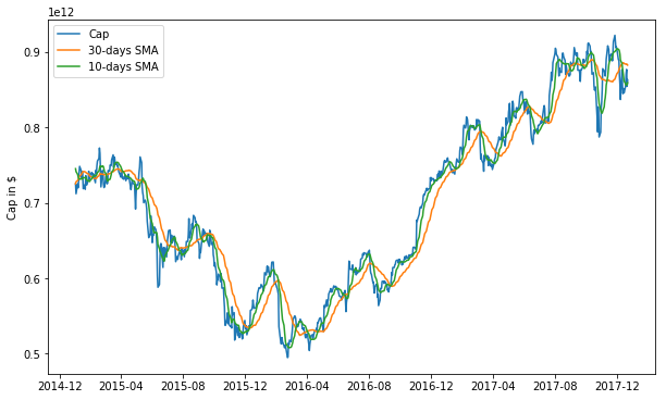
Here we provide a “warm start” by computing two simple moving average signals that you can use as benchmark in your analysis.
Generate moving averages
# Calculating the short-window (10 days) simple moving average

window_1 = 10

short_rolling = df_cap.rolling(window=window_1).mean()
# short_rolling.head(20)
# Calculating the long-window (30 days) simple moving average

window_2 = 30
long_rolling = df_cap.rolling(window=window_2).mean()
# long_rolling.tail()
Plot three years of AAPL stock:
ticker = 'AAPL'
start_date = '2015-01-01'
end_date = '2017-12-31'

fig = plt.figure(figsize=(10,6))
ax = fig.add_subplot(1,1,1)

ax.plot(df_cap.loc[start_date:end_date, :].index, df_cap.loc[start_date:end_date, 'AAPL'], label='Cap')
ax.plot(long_rolling.loc[start_date:end_date, :].index, long_rolling.loc[start_date:end_date, 'AAPL'],
          label = '%d-days SMA' % window_2)
ax.plot(short_rolling.loc[start_date:end_date, :].index, short_rolling.loc[start_date:end_date, 'AAPL'],
         label = '%d-days SMA' % window_1)

ax.legend(loc='best')
ax.set_ylabel('Cap in $')

plt.show()
Part 1: Model calibration with moving average signals (Max 10 points)
Recall the equation for the dynamics of market portfolio:
\[\Delta {\bf x}_t = \kappa_x \circ {\bf x}_t \circ \left( {\bf W}{\bf z}_t' - {\bf x}_t \right) + {\bf x}_t \circ \varepsilon_t^{(x)}\]Here we change the notation a bit. Now \({\bf z}_t'\) is an extended vector of predictors that includes a constant unit predictor \({\bf z}_t' = [1, {\bf z}_t ]^T\). Therefore, for each name, if you have \(K = 2\) signals, an extended vector of signals \({\bf z}_t'\) is of length \(K + 1\), and the \(W\) stands for a factor loading matrix. The negative log-likelihood function for observable data with this model is therefore
\[LL_M (\Theta) = - \log \prod_{t=0}^{T-1} \frac{1}{ \sqrt{ (2 \pi)^{N} \left| \Sigma_x \right| }} e^{ - \frac{1}{2} \left( {\bf v}_t \right)^{T} \Sigma_x^{-1} \left( {\bf v}_t \right)}\]where
and \(\Sigma_x\) is the covariance matrix that was specified above in terms of other parameters. Here we directly infer the value of \(\Sigma_x\), along with other parameters, from data, so we will not use these previous expressions.
Parameters that you have to estimate from data are therefore the vector of mean reversion speed parameters \(\kappa_x\), factor loading matrix \({\bf W} \equiv {\bf w}_z'\), and covariance matrix \(\Sigma_x\).
Now, you are free to impose some structure on this parameters. Here are some choice, in the order of increasing complexity:
-
assume that all values in vector-valued and matrix-valued parameters are the same, so that they can parametrized by scalars, e.g. \(\kappa_x = \kappa {\bf 1}_N\) where \(\kappa\) is a scalar value, and \({\bf 1}_N\) is a vector of ones of length \(N\) where \(N\) is the number of stocks in the market portfolio. You can proceed similarly with specification of factor loading matrix \(W'\). Assume that all values in (diagonal!) factor loading matrices are the same for all names, and assume that all correlations and variances in the covariance matrix \(\Sigma_x\) are the same for all names.
-
Assume that all values are the same only within a given industrial sector.
-
You can also change the units. For example, you can consider logs of market caps instead of market caps themselves, ie. change the variable from \({\bf x}_t\) to \({\bf q}_t = \log {\bf x}_t\)
Data Preparation
# Manipulate raw data
# NOTE: .sum() has axis 1 because we want the sum of the column which is just
#       1 ticker symbol.
#       .mean() will then take the mean average of all the ticker symbol
average_market_cap = df_cap.sum(axis=1).mean()

# Average
short_rolling_average = short_rolling / average_market_cap
long_rolling_average = long_rolling / average_market_cap
df_cap_average = df_cap / average_market_cap
#
# By looking at the debug cells below, we see that both heads for the long and short de-meaned pandas Dataframes have NaN
# (Not-a-number.)
# Going to only start with the first valid number
# Using .first_valid_index
# https://stackoverflow.com/questions/42137529/pandas-find-first-non-null-value-in-column
short_rolling_average_first_valid = (short_rolling_average
                                    /
                                    short_rolling_average.loc[ short_rolling_average.first_valid_index() ])
long_rolling_average_first_valid = (long_rolling_average
                                   /
                                   long_rolling_average.loc[ long_rolling_average.first_valid_index() ])


# De-mean
# https://www.youtube.com/watch?v=E5PZR4YpBtM
short_rolling_demeaned = short_rolling_average_first_valid.pct_change(periods=1).shift(-1)
long_rolling_demeaned = long_rolling_average_first_valid.pct_change(periods=1).shift(-1)
# DEBUG
#
type(short_rolling_average)
pandas.core.frame.DataFrame
# Clean data

# Drop last row
market_cap = df_cap_average[:-1]

# Drop not-a-numbers
signal_1 = short_rolling_demeaned.copy()
signal_2 = long_rolling_demeaned.copy()
#
signal_1 = signal_1.dropna()
signal_2 = signal_2.dropna()

# # Get rid rows where dates that do not match
market_cap = market_cap[ market_cap.index.isin(signal_1.index) & market_cap.index.isin(signal_2.index)]
signal_1 = signal_1[signal_1.index.isin( market_cap.index )]
signal_2 = signal_2[signal_2.index.isin( market_cap.index )]
# Get the amount of time steps
t = market_cap.shape[0]
t
2050
# Get the number of stocks
n = market_cap.shape[1]
n
30
Calibration with Tensorflow
start_date = '2010-1-1'
end_date = '2017-12-31'

# Only get the dates required
market_cap_focused = market_cap.loc[ start_date : end_date ]
signal_1_focused = signal_1.loc[ start_date : end_date ]
signal_2_focused = signal_2.loc[ start_date : end_date ]

# Mentioned in the instructions, 2 signals means k = 2
k = 2
# Creating a Pandas Dataframe to hold the results
results = pd.DataFrame( [],
                        index = market_cap_focused.columns,
                        columns = [ 'kappa',
                                    'sigma',
                                    'sigma^2',
                                    'w1',
                                    'w2'] )
# Tensorflow graph
tf.reset_default_graph()

# Input
x = tf.placeholder( shape = (None, n),
                    dtype = tf.float32,
                    name = 'x' )

# Signals
z1  = tf.placeholder( shape = (None,n),
                      dtype = tf.float32,
                      name = 'z1' )
z2  = tf.placeholder( shape = ( None, n),
                      dtype=tf.float32,
                      name = 'z2' )

# Variables
N_k = n
N_s = n
N_w = n
kappa = tf.get_variable( "kappa",
                         initializer = tf.random_uniform(
                                             [N_k],
                                             minval = 0.0,
                                             maxval = 1.0) )
sigma = tf.get_variable( "sigma",
                         initializer = tf.random_uniform(
                                             [N_s],
                                             minval=0.0,
                                             maxval=0.1) )

# Weights

#-------------------
w1_init = tf.random_normal( [N_w],
                            mean=0.5,
                            stddev=0.1 )
w2_init = 1 - w1_init
w1 = tf.get_variable( "w1",
                      initializer = w1_init)
w2 = tf.get_variable( "w2",
                      initializer=w2_init )

W1 = w1*tf.ones(n)
W2 = w2*tf.ones(n)


# Gaussian
#-------------------
mu    = tf.zeros( [n] )
Sigma = sigma*tf.ones( [n] )
theta1 = tf.multiply( W1,
                      z1)
theta2 = tf.multiply( W2,
                      z2)
scale  = tf.slice( x,
                   [0,0],
                   [1,-1] )
theta  = tf.multiply( scale,
                      tf.cumprod( 1 + tf.add( theta1,
                                              theta2) ) )

Kappa = kappa*tf.ones( [n] )

r = tf.divide( tf.subtract( tf.manip.roll( x,
                                           shift = -1,
                                           axis = 0),
                            x),
               x)
v = tf.subtract( r,
                 tf.multiply( Kappa,
                              tf.subtract( theta,
                                           x) ) )
# NOTE: Do not use last row
vuse = tf.slice( v,
                 [0,0],
                 [tf.shape(v)[0]-1,-1] )

#  Constraint - No negative
#-------------------
clip_w1 = w1.assign(tf.maximum(0., w1))
clip_w2 = w2.assign(tf.maximum(0., w2))
clip = tf.group(clip_w1, clip_w2)

dist = tf.contrib.distributions.MultivariateNormalDiag(loc=mu, scale_diag=Sigma)
log_prob = dist.log_prob(vuse)
reg_term = tf.reduce_sum(tf.square(w1+w2-1))
neg_log_likelihood = -tf.reduce_sum(log_prob) + 0.01*reg_term

# Optimizer
#-------------------
optimizer = tf.train.AdamOptimizer(learning_rate=0.0001)
train_op = optimizer.minimize( neg_log_likelihood )
WARNING:tensorflow:From <ipython-input-22-bc07b1883c93>:85: MultivariateNormalDiag.__init__ (from tensorflow.contrib.distributions.python.ops.mvn_diag) is deprecated and will be removed after 2018-10-01.
Instructions for updating:
The TensorFlow Distributions library has moved to TensorFlow Probability (https://github.com/tensorflow/probability). You should update all references to use `tfp.distributions` instead of `tf.contrib.distributions`.
WARNING:tensorflow:From /opt/conda/lib/python3.6/site-packages/tensorflow/contrib/distributions/python/ops/mvn_diag.py:223: MultivariateNormalLinearOperator.__init__ (from tensorflow.contrib.distributions.python.ops.mvn_linear_operator) is deprecated and will be removed after 2018-10-01.
Instructions for updating:
The TensorFlow Distributions library has moved to TensorFlow Probability (https://github.com/tensorflow/probability). You should update all references to use `tfp.distributions` instead of `tf.contrib.distributions`.
WARNING:tensorflow:From /opt/conda/lib/python3.6/site-packages/tensorflow/contrib/distributions/python/ops/mvn_linear_operator.py:200: AffineLinearOperator.__init__ (from tensorflow.contrib.distributions.python.ops.bijectors.affine_linear_operator) is deprecated and will be removed after 2018-10-01.
Instructions for updating:
The TensorFlow Distributions library has moved to TensorFlow Probability (https://github.com/tensorflow/probability). You should update all references to use `tfp.distributions` instead of `tf.contrib.distributions`.
WARNING:tensorflow:From /opt/conda/lib/python3.6/site-packages/tensorflow/contrib/distributions/python/ops/bijectors/affine_linear_operator.py:158: _DistributionShape.__init__ (from tensorflow.contrib.distributions.python.ops.shape) is deprecated and will be removed after 2018-10-01.
Instructions for updating:
The TensorFlow Distributions library has moved to TensorFlow Probability (https://github.com/tensorflow/probability). You should update all references to use `tfp.distributions` instead of `tf.contrib.distributions`.
max_iteration = 5000
tolerence = 1e-15
# Save Tensorflow model because running the weight
saver = tf.train.Saver()

# Run Tensorflow
with tf.Session() as sess:
    sess.run(tf.global_variables_initializer())

    losses = sess.run([neg_log_likelihood], feed_dict={x: market_cap_focused, z1: signal_1_focused, z2: signal_2_focused})
    i=1

    # Calibrate print out
    print( "------------------- Calibration Calculating ----------------------" )
    print(" iter |       Loss       |   difference")

    while True:

        sess.run(train_op, feed_dict={x: market_cap_focused, z1: signal_1_focused, z2: signal_2_focused})
        sess.run(clip) # force weights to be non-negative

        # update loss
        new_loss = sess.run(neg_log_likelihood, feed_dict={x: market_cap_focused, z1: signal_1_focused, z2: signal_2_focused})
        loss_diff = np.abs(new_loss - losses[-1])
        losses.append(new_loss)

        if i%min(1000,(max_iteration/20))==1:
            print ("{:5} | {:16.4f} | {:12.4f}".format(i,new_loss,loss_diff))

        if loss_diff < tolerence:
            print('Loss function convergence in {} iterations!'.format(i))
            print('Old loss: {}  New loss: {}'.format(losses[-2],losses[-1]))
            break

        if i >= max_iteration:
            print('Max number of iterations reached without convergence.')
            break

        i += 1

    # Put data in pandas Dataframe.
    results['kappa'] = sess.run(kappa)
    results['sigma'] = sess.run(sigma)
    results['sigma^2'] = sess.run(sigma)**2
    results['w1'] = sess.run(W1)
    results['w2'] = sess.run(W2)

    fitted_means = sess.run(theta, feed_dict={x: market_cap_focused, z1: signal_1_focused, z2: signal_2_focused})
    mean_levels = pd.DataFrame(fitted_means,index=market_cap_focused.index,columns=market_cap_focused.columns)


    print( "------------------- Calibration Results ----------------------" )
    print(results.round(4))


    save_path = saver.save(sess, './part01_model.ckpt')
    print( 'Model saved in path: {}'.format(save_path) )
------------------- Calibration Calculating ----------------------
 iter |       Loss       |   difference
    1 |     2327035.0000 | 8970866.0000
  251 |      -82114.7656 |     251.0469
  501 |     -126741.5547 |     111.5469
  751 |     -142108.1719 |      38.8750
 1001 |     -149853.1250 |      24.7500
 1251 |     -155012.7344 |      17.2188
 1501 |     -158718.5938 |      12.6875
 1751 |     -161523.0156 |       9.8281
 2001 |     -163727.9531 |       7.9219
 2251 |     -165512.4531 |       6.4844
 2501 |     -166989.7344 |       5.3438
 2751 |     -168235.1406 |       4.6250
 3001 |     -169300.4531 |       3.9844
 3251 |     -170222.7344 |       3.4531
 3501 |     -171029.1250 |       2.9844
 3751 |     -171739.5000 |       2.6719
 4001 |     -172369.7500 |       2.4062
 4251 |     -172932.1875 |       2.1094
 4501 |     -173436.4375 |       1.9375
 4751 |     -173890.0469 |       1.7500
Max number of iterations reached without convergence.
------------------- Calibration Results ----------------------
       kappa   sigma  sigma^2      w1      w2
AAPL  0.5439  0.0157   0.0002  0.9817  0.0000
AXP   1.0526  0.0146   0.0002  0.7656  0.1791
BA    0.6858  0.0149   0.0002  0.4264  0.5904
CAT   0.8151  0.0166   0.0003  0.9467  0.0000
CSCO  0.6793  0.0160   0.0003  0.8691  0.0525
CVX   1.0397  0.0134   0.0002  0.9572  0.0000
DIS   0.6507  0.0135   0.0002  0.9929  0.0000
DWDP  0.9293  0.0273   0.0007  1.0093  0.0000
GE    0.7334  0.0140   0.0002  0.8600  0.1223
GS    1.0504  0.0167   0.0003  0.6647  0.1298
HD    0.6671  0.0126   0.0002  0.9596  0.0400
IBM   0.6618  0.0123   0.0002  0.8662  0.0736
INTC  1.1348  0.0148   0.0002  0.9204  0.0000
JNJ   1.3547  0.0097   0.0001  0.9896  0.0000
JPM   1.1444  0.0163   0.0003  0.9732  0.0000
KO    1.1623  0.0091   0.0001  0.7522  0.2208
MCD   0.9231  0.0096   0.0001  1.0175  0.0000
MMM   1.1913  0.0115   0.0001  0.9998  0.0000
MRK   1.4140  0.0121   0.0001  0.9643  0.0000
MSFT  1.2031  0.0142   0.0002  0.9616  0.0427
NKE   1.2191  0.0149   0.0002  0.5916  0.4270
PFE   0.5548  0.0117   0.0001  0.6836  0.4084
PG    0.1084  0.0035   0.0000  0.3463  0.4518
TRV   0.7244  0.0115   0.0001  0.8661  0.0000
UNH   1.1193  0.0142   0.0002  0.5058  0.5468
UTX   0.6846  0.0123   0.0002  1.0128  0.0000
V     0.9229  0.0151   0.0002  0.8900  0.1141
VZ    0.5464  0.0144   0.0002  0.9873  0.0124
WMT   0.9592  0.0109   0.0001  0.9649  0.0000
XOM   1.1643  0.0117   0.0001  0.9337  0.0000
Model saved in path: ./part01_model.ckpt
# Save the dataframe
results.to_csv('df_results_part01.csv')
results.to_csv('df_mean_levels_part01.csv')
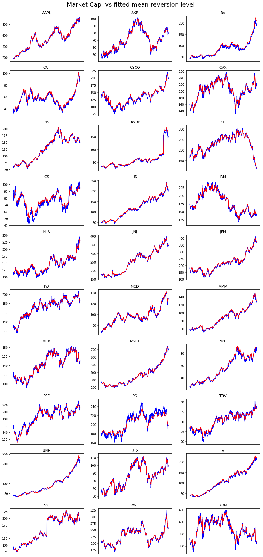
Plot Martket Cap against Fitted Mean Reversion Level
data = df_cap
theta = mean_levels
start_date='2010-01-01'
end_date='2017-12-31'
nplot = 30
scale = 1
title = 'Market Cap '

avg_mkt_cap = data.sum(axis=1).mean() # average market cap over the period

N = data.shape[1]


if N > nplot: N = nplot

plt.figure(figsize=(15,N))
plt.suptitle(title + ' vs fitted mean reversion level',size=20)
ytop = 0.96-0.4*np.exp(-N/5)
plt.subplots_adjust(top=ytop)

stocks = data.columns[:N]
for index, stock in enumerate(stocks,1):
    plt.subplot(np.ceil(N/3),3,index)
    plt.plot(scale*(1/1e9)*data.loc[start_date:end_date][stock],color='blue',label='Market cap ($Bn)')
    plt.plot(scale*(avg_mkt_cap/1e9)*theta.loc[start_date:end_date][stock],color='red',label='Mean reversion level')
    plt.title(stock,size=12)
    plt.xticks([])
plt.show()
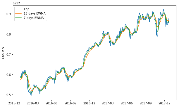
Part 2: Propose and analyse your own signals (Max 10 points)
In this part, you will experiment with other signals. Propose a signal and explain why it is interesting to include this signal in the portfolio analysis. Then add your favorite signal or signals to the previous benchmarck signals (or alternatively you can replace them), and repeat the analysis of model calibration. State your conclusions.
# Put the rest of your code and analysis for Part 2 here.
exp_wgt_mov_avg_window_a = 7
exp_wgt_mov_avg_window_b = 15

# https://pandas.pydata.org/pandas-docs/stable/generated/pandas.DataFrame.ewm.html
# Provides exponential weighted functions
# Then you take the .mean() to get the average.
exp_wgt_mov_avg_short = df_cap.ewm( span = exp_wgt_mov_avg_window_a,
                                              adjust = False ).mean()
exp_wgt_mov_avg_long = df_cap.ewm( span = exp_wgt_mov_avg_window_b,
                                             adjust = False ).mean()
# This is similar code as the cell above but instead of 3 years of stock info, just using 2 years.
# Also changing rolling to exponential weighted moving average (left the original commented out.)
ticker = 'AAPL'
start_date = '2016-01-01'
end_date = '2017-12-31'

fig = plt.figure(figsize=(10,6))
ax = fig.add_subplot(1,1,1)

ax.plot(df_cap.loc[start_date:end_date, :].index, df_cap.loc[start_date:end_date, 'AAPL'], label='Cap')
# ax.plot(long_rolling.loc[start_date:end_date, :].index, long_rolling.loc[start_date:end_date, 'AAPL'],
#           label = '%d-days SMA' % window_2)
ax.plot(exp_wgt_mov_avg_long.loc[start_date:end_date, :].index, exp_wgt_mov_avg_long.loc[start_date:end_date, 'AAPL'],
            label = '%d-days EWMA' % exp_wgt_mov_avg_window_b)
ax.plot(exp_wgt_mov_avg_short.loc[start_date:end_date, :].index, exp_wgt_mov_avg_short.loc[start_date:end_date, 'AAPL'],
         label = '%d-days EWMA' % exp_wgt_mov_avg_window_a)

ax.legend(loc='best')
ax.set_ylabel('Cap in $')

plt.show()
Data Preparation
# Manipulate raw data
# NOTE: .sum() has axis 1 because we want the sum of the column which is just
#       1 ticker symbol.
#       .mean() will then take the mean average of all the ticker symbol
average_market_cap = df_cap.sum(axis=1).mean()

# Average
short_ewma_average = exp_wgt_mov_avg_short / average_market_cap
long_ewma_average = exp_wgt_mov_avg_long / average_market_cap
df_cap_average = df_cap / average_market_cap
#
# By looking at the debug cells below, we see that both heads for the long and short de-meaned pandas Dataframes have NaN
# (Not-a-number.)
# Going to only start with the first valid number
# Using .first_valid_index
# https://stackoverflow.com/questions/42137529/pandas-find-first-non-null-value-in-column
short_ewma_average_first_valid = (short_ewma_average
                                    /
                                    short_ewma_average.loc[ short_ewma_average.first_valid_index() ])
long_ewma_average_first_valid = (long_ewma_average
                                   /
                                   long_ewma_average.loc[ long_ewma_average.first_valid_index() ])

# De-mean
# https://www.youtube.com/watch?v=E5PZR4YpBtM
short_ewma_demeaned = short_ewma_average_first_valid.pct_change(periods=1).shift(-1)
long_ewma_demeaned = long_ewma_average_first_valid.pct_change(periods=1).shift(-1)
# Clean data

# Drop last row
market_cap = df_cap_average[:-1]

# Drop not-a-numbers
signal_1 = short_ewma_demeaned.copy()
signal_2 = long_ewma_demeaned.copy()
#
signal_1 = signal_1.dropna()
signal_2 = signal_2.dropna()

# # Get rid rows where dates that do not match
market_cap = market_cap[ market_cap.index.isin(signal_1.index) & market_cap.index.isin(signal_2.index)]
signal_1 = signal_1[signal_1.index.isin( market_cap.index )]
signal_2 = signal_2[signal_2.index.isin( market_cap.index )]
# Get the amount of time steps
t = market_cap.shape[0]
t
2079
# Get the number of stocks
n = market_cap.shape[1]
n
30
Calibration with Tensorflow
start_date = '2010-1-1'
end_date = '2017-12-31'

# Only get the dates required
market_cap_focused = market_cap.loc[ start_date : end_date ]
signal_1_focused = signal_1.loc[ start_date : end_date ]
signal_2_focused = signal_2.loc[ start_date : end_date ]

# Mentioned in the instructions, 2 signals means k = 2
k = 2
# Creating a Pandas Dataframe to hold the results
results = pd.DataFrame( [],
                        index = market_cap_focused.columns,
                        columns = [ 'kappa',
                                    'sigma',
                                    'sigma^2',
                                    'w1',
                                    'w2'] )
# Tensorflow graph
tf.reset_default_graph()

# Input
x = tf.placeholder( shape = (None, n),
                    dtype = tf.float32,
                    name = 'x' )

# Signals
z1  = tf.placeholder( shape = (None,n),
                      dtype = tf.float32,
                      name = 'z1' )
z2  = tf.placeholder( shape = ( None, n),
                      dtype=tf.float32,
                      name = 'z2' )

# Variables
N_k = n
N_s = n
N_w = n
kappa = tf.get_variable( "kappa",
                         initializer = tf.random_uniform(
                                             [N_k],
                                             minval = 0.0,
                                             maxval = 1.0) )
sigma = tf.get_variable( "sigma",
                         initializer = tf.random_uniform(
                                             [N_s],
                                             minval=0.0,
                                             maxval=0.1) )

# Weights
#-------------------
w1_init = tf.random_normal( [N_w],
                            mean=0.5,
                            stddev=0.1 )
w2_init = 1 - w1_init
w1 = tf.get_variable( "w1",
                      initializer = w1_init)
w2 = tf.get_variable( "w2",
                      initializer=w2_init )

W1 = w1*tf.ones(n)
W2 = w2*tf.ones(n)


# Gaussian
#-------------------
mu    = tf.zeros( [n] )
Sigma = sigma*tf.ones( [n] )
theta1 = tf.multiply( W1,
                      z1)
theta2 = tf.multiply( W2,
                      z2)
scale  = tf.slice( x,
                   [0,0],
                   [1,-1] )
theta  = tf.multiply( scale,
                      tf.cumprod( 1 + tf.add( theta1,
                                              theta2) ) )

Kappa = kappa*tf.ones( [n] )

r = tf.divide( tf.subtract( tf.manip.roll( x,
                                           shift = -1,
                                           axis = 0),
                            x),
               x)
v = tf.subtract( r,
                 tf.multiply( Kappa,
                              tf.subtract( theta,
                                           x) ) )
# NOTE: Do not use last row
vuse = tf.slice( v,
                 [0,0],
                 [tf.shape(v)[0]-1,-1] )

#  Constraint - No negative
#-------------------
clip_w1 = w1.assign(tf.maximum(0., w1))
clip_w2 = w2.assign(tf.maximum(0., w2))
clip = tf.group(clip_w1, clip_w2)

dist = tf.contrib.distributions.MultivariateNormalDiag(loc=mu, scale_diag=Sigma)
log_prob = dist.log_prob(vuse)
reg_term = tf.reduce_sum(tf.square(w1+w2-1))
neg_log_likelihood = -tf.reduce_sum(log_prob) + 0.01*reg_term

# Optimizer
#-------------------
optimizer = tf.train.AdamOptimizer(learning_rate=0.0001)
train_op = optimizer.minimize( neg_log_likelihood )
max_iteration = 5000
tolerence = 1e-15
# Save Tensorflow model because running the weight
saver = tf.train.Saver()

# Run Tensorflow
with tf.Session() as sess:
    sess.run(tf.global_variables_initializer())

    losses = sess.run([neg_log_likelihood], feed_dict={x: market_cap_focused, z1: signal_1_focused, z2: signal_2_focused})
    i=1

    # Calibrate print out
    print( "------------------- Calibration Calculating ----------------------" )
    print(" iter |       Loss       |   difference")

    while True:

        sess.run(train_op, feed_dict={x: market_cap_focused, z1: signal_1_focused, z2: signal_2_focused})
        sess.run(clip) # force weights to be non-negative

        # update loss
        new_loss = sess.run(neg_log_likelihood, feed_dict={x: market_cap_focused, z1: signal_1_focused, z2: signal_2_focused})
        loss_diff = np.abs(new_loss - losses[-1])
        losses.append(new_loss)

        if i%min(1000,(max_iteration/20))==1:
            print ("{:5} | {:16.4f} | {:12.4f}".format(i,new_loss,loss_diff))

        if loss_diff < tolerence:
            print('Loss function convergence in {} iterations!'.format(i))
            print('Old loss: {}  New loss: {}'.format(losses[-2],losses[-1]))
            break

        if i >= max_iteration:
            print('Max number of iterations reached without convergence.')
            break

        i += 1

    # Put data in pandas Dataframe.
    results['kappa'] = sess.run(kappa)
    results['sigma'] = sess.run(sigma)
    results['sigma^2'] = sess.run(sigma)**2
    results['w1'] = sess.run(W1)
    results['w2'] = sess.run(W2)

    fitted_means = sess.run(theta, feed_dict={x: market_cap_focused, z1: signal_1_focused, z2: signal_2_focused})
    mean_levels = pd.DataFrame(fitted_means,index=market_cap_focused.index,columns=market_cap_focused.columns)


    print( "------------------- Calibration Results ----------------------" )
    print(results.round(4))


    save_path = saver.save(sess, './part02_model.ckpt')
    print( 'Model saved in path: {}'.format(save_path) )
------------------- Calibration Calculating ----------------------
 iter |       Loss       |   difference
    1 |      145405.3594 |   72699.7812
  251 |     -146791.0312 |     144.2344
  501 |     -171243.8594 |      55.9688
  751 |     -177963.1406 |       4.2031
 1001 |     -178767.1094 |       2.4219
 1251 |     -179266.0156 |       1.6406
 1501 |     -179604.4844 |       1.1406
 1751 |     -179848.3438 |       0.9062
 2001 |     -180031.5938 |       0.6562
 2251 |     -180173.8594 |       0.5156
 2501 |     -180287.2344 |       0.4062
 2751 |     -180379.4688 |       0.3594
 3001 |     -180455.7812 |       0.2188
 3251 |     -180519.5781 |       0.2344
 3501 |     -180573.5625 |       0.1875
 3751 |     -180620.0938 |       0.1875
 4001 |     -180660.5781 |       0.1719
 4251 |     -180696.2344 |       0.1250
 4501 |     -180727.7344 |       0.0938
 4751 |     -180754.7812 |       0.1094
Loss function convergence in 4960 iterations!
Old loss: -180774.90625  New loss: -180774.90625
------------------- Calibration Results ----------------------
       kappa   sigma  sigma^2      w1      w2
AAPL  1.0758  0.0155   0.0002  1.0040  0.0000
AXP   1.2289  0.0147   0.0002  1.0064  0.0000
BA    0.5584  0.0137   0.0002  0.6606  0.4096
CAT   1.1496  0.0168   0.0003  1.0395  0.0000
CSCO  1.4412  0.0158   0.0003  0.9616  0.0146
CVX   1.0059  0.0133   0.0002  0.9989  0.0000
DIS   1.0815  0.0134   0.0002  1.0073  0.0000
DWDP  1.1490  0.0273   0.0007  0.8781  0.1595
GE    1.1903  0.0139   0.0002  0.9999  0.0000
GS    1.4177  0.0167   0.0003  0.9267  0.0000
HD    1.3413  0.0126   0.0002  0.7823  0.2292
IBM   1.1469  0.0122   0.0001  0.9896  0.0000
INTC  0.6429  0.0148   0.0002  0.8633  0.1856
JNJ   1.5356  0.0096   0.0001  0.8211  0.1844
JPM   1.2158  0.0163   0.0003  1.0150  0.0000
KO    1.4280  0.0091   0.0001  0.9566  0.0472
MCD   0.7257  0.0096   0.0001  0.6767  0.3586
MMM   0.7104  0.0115   0.0001  0.9223  0.1122
MRK   0.5685  0.0122   0.0001  0.9950  0.0000
MSFT  0.6107  0.0142   0.0002  0.7523  0.2699
NKE   0.5885  0.0149   0.0002  0.8673  0.1892
PFE   0.6223  0.0117   0.0001  0.9907  0.0107
PG    1.3555  0.0089   0.0001  0.9005  0.0935
TRV   0.8703  0.0115   0.0001  1.0048  0.0000
UNH   1.1124  0.0142   0.0002  0.8014  0.2204
UTX   1.1390  0.0123   0.0002  1.0049  0.0000
V     1.1783  0.0150   0.0002  1.0169  0.0000
VZ    1.1977  0.0143   0.0002  0.9020  0.1030
WMT   1.4701  0.0107   0.0001  0.9971  0.0000
XOM   1.1844  0.0116   0.0001  0.9369  0.0533
Model saved in path: ./part02_model.ckpt
# Save the dataframe
results.to_csv('df_results_part02.csv')
results.to_csv('df_mean_levels_part02.csv')
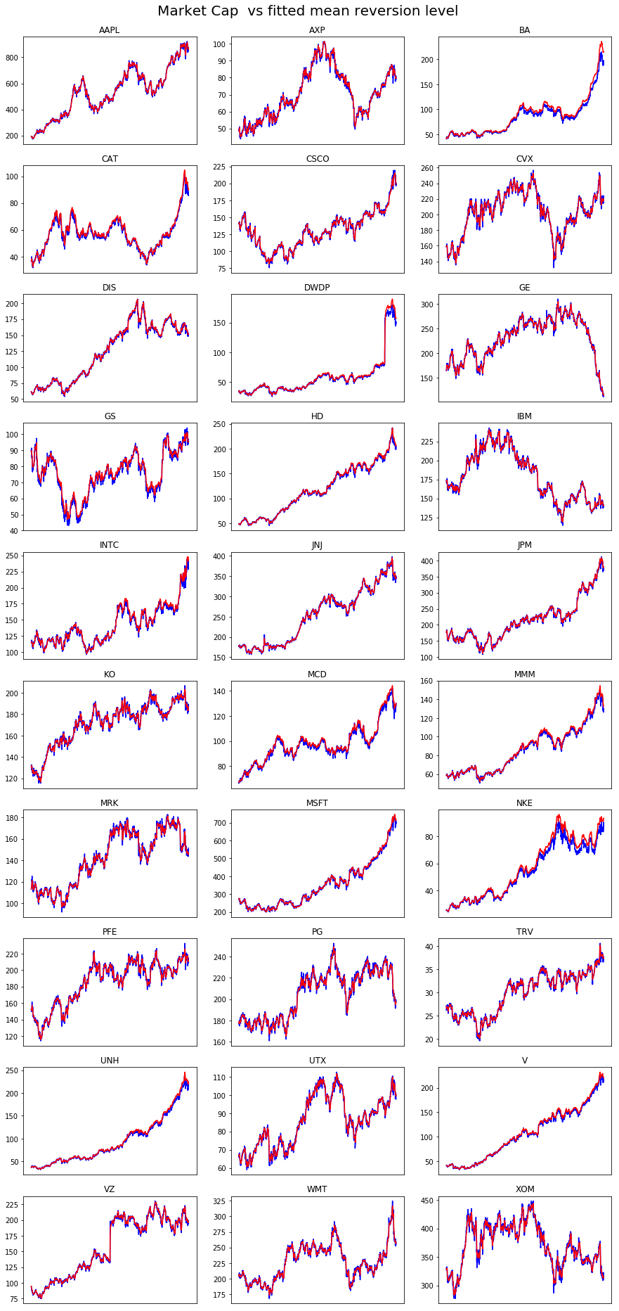
data = df_cap
theta = mean_levels
start_date='2010-01-01'
end_date='2017-12-31'
nplot = 30
scale = 1
title = 'Market Cap '

avg_mkt_cap = data.sum(axis=1).mean() # average market cap over the period

N = data.shape[1]


if N > nplot: N = nplot

plt.figure(figsize=(15,N))
plt.suptitle(title + ' vs fitted mean reversion level',size=20)
ytop = 0.96-0.4*np.exp(-N/5)
plt.subplots_adjust(top=ytop)

stocks = data.columns[:N]
for index, stock in enumerate(stocks,1):
    plt.subplot(np.ceil(N/3),3,index)
    plt.plot(scale*(1/1e9)*data.loc[start_date:end_date][stock],color='blue',label='Market cap ($Bn)')
    plt.plot(scale*(avg_mkt_cap/1e9)*theta.loc[start_date:end_date][stock],color='red',label='Mean reversion level')
    plt.title(stock,size=12)
    plt.xticks([])
plt.show()
Part 3: Can you do it for the S&P500 market portfolio? (Max 10 point)
Try to repeat your analysis for the S&P500 portfolio.
The data can be obtained from Course 2 “Fundamentals of Machine Learning in Finance” in this Specialization.
# Put the rest of your code and analysis for Part 3 here.
Part 4 (Optional): Show me something else.
Here you can develop any additional analysis of the model that you may find interesting (One possible suggestion is presented above, but you should feel free to choose your own topic). Present your case and finding/conclusions.
# Put the rest of your code and analysis for Part 3 here.